Aberrations

Introduction

A perfect imaging system can image a point into a point. However, any imaging system has some flaws which degrade the image quality, and therefore a point is not imaged to a perfect point but into a larger spot. When these flews caused by the optical element they are called aberrations, and there are different types of aberrations which are leading to different types of spots. Here, we will focus on the three most common types of aberrations: coma, spherical, and chromatic. 

These aberrations lower the resolution of imaging systems and make it challenging to build a microscope or a telescope since the aberrations increases when increasing the magnification. However, once different techniques were developed to overcome these aberrations, new paths of research were opened.  Most of these techniques are based on resorting to several elements with the opposite value of aberration so they cancel each other.

A perfect lens has a parabolic shape so it imposes a quadratic phase on the incoming wave and is infinitely large. This lens focuses an input plane wave toward a single point at the focus or it can image a point object into a point when satisfying the imaging condition:

\frac1u+\frac1v=\frac1f

Where u is the distance between the lens and the object, v is the distance between the lens and the image, and f is the focal length of the lens. According to geometrical optics, a point source will result in a point image. This is illustrated in Fig. 1.

Fig. 1. Focusing plane-wave with a plano-convex lens and measuring the focal plane.
Fig. 2. Measured spot side at the focal plane showing a point as small as the detector resolution.

However, even with a perfect lens, a point source will not lead to a point image but to a blur disk. This blur disk is called the Point Spread Function (PSF) and it indicates the spatial resolution of the imaging system.  This is due to the finite lens aperture leading to some of the beams leaving the point source and missing the lens. Therefore, the resolution of an image is a function of the aperture size of the lens or the imaging system. If the lens is perfect, without any aberrations, the image size of a point source, namely the PSF, is:

PSF=\frac{4\lambda\nu}{\pi D}

Where D is the lens aperture, v is the distance to the image, and \lambda is the wavelength. As evident, when we increase the size of the lens, the PSF is smaller, meaning a better resolution. Also, getting close to the lens and reducing v is improving the resolution. However, even if the lens is infinitely large and all the light from the point source is entering the lens, the image cannot be smaller than half the wavelength due to the wave aspect of the light. This is also seen in the wavelength-dependent function. Reducing the wavelength will reduce the PSF and will improve the resolution. However, to observe these effects, we must leave the geometrical optics and consider wave optics.

Defocus

The most common type of aberration is defocusing. In defocus the image is out of focus since the detector is not situated exactly at the image plane. In this case, a point object generates a larger blur disk, namely, we have a larger PSF, which leads to a reduction in the image resolution. This is shown in Fig. 3 where we shifted the detector from the exact focal plane. The size of the PSF as a function of distance from the image plane, z, is:

PSF(z)=PSF(0)\sqrt{1+{(\frac{z\lambda}{\pi PSF{(0)}^2})}^2}

Here, the size of the PSF is slowly increasing when z is small, but when z is large it is linearly increasing with z. Thus, there is a range where the PSF is not affected even if we are slightly out-of-focus. This range is called the Rayleigh range and it sets what is the depth of focus of our system. If the depth of focus is large, we do not need to be so accurate, and different objects at different distances can still be in focus. However, when the depth of focus is small, only one object will be in focus, leading to beautiful images of a sharp object with a blurred background. The depth of focus, b, is calculated by

b=\frac{\pi PSF{(0)}^2}{2\lambda}

Therefore, a smaller spot is leading to a smaller depth of focus. So, when the aperture is large we have a higher resolution with a lower depth of focus. 

Defocusing is a type of aberration that is easily fixed by changing the position of the detector or by changing the position of the lens. In some cases, it is also possible to change the curvature of the lens. This is how our eye is focusing and defocusing on different objects.

Fig. 3. Measured spot size when the detector is shifted from the correct distance. As shown, the spot is larger than the one measured in the focal plane (Fig. 2).

Tilt

The second type of aberration is when the detector is not oriented according to the image plane. This leads to a PSF which is a function of the position in the plane. The resolution can be high in the center of the image and then it will be lower resolution along a specific axis. If the tilt is large enough, the PSF will change into an asymmetric ellipse as shown in Fig. 4. We can define the tilt according to Zernike polynomials:

T_x\;=\;A_x\cos(\alpha)\\T_y\;=\;A_y\sin(\alpha)

Therefore, this type of aberration is also easy to fix by orienting the detector correctly, along the image plane.

Fig. 4. Measurements of a PSF by a tilted detector showing an asymmetric ellipse.

Spherical aberrations

Many times, the facet of lenses does not have a parabolic shape but is more similar to a spherical shape which is easier to fabricate. These circular facets in 2d are described by: I need to make here a figure showing the lens curvature as a function of x,y, and doing the paraxial approximation.

\triangle z(x,y)=R-\sqrt{R^2-X^2-Y^2}=R(1-\sqrt{1-\frac{r^2}{R^2})}

Where z is the optical axis, x and y are the transverse axes, and r^2=x^2+y^2. When the lens is thin and we interact with the center of the lens, this equation can be approximated according to the paraxial approximation:

r^2<<R^2

leading to:

\triangle z=\frac{r^2}{2R^2}+O(r^4)

This quadratic thickness imposes a quadratic phase on the input beam which leads to all the lens properties of focusing and imaging. The higher terms at the order of O(r^4) are leading to aberrations known as spherical aberrations. These aberrations start to be significant when the lens is large, when its curvature is high, or when considering small objects, where even small aberrations are influencing the resulting image. The r^3 term is usually zero since the lens has cylindrical symmetry.

The main effect of spherical aberrations is that the focal length is not constant across the lens but depends on the distance from the center of the lens, r. We can calculate the local focal length as a function of r, as:

\frac1{f(r)}\cong\frac2R+\frac{3r^2}{2R^3}

This is shown in Fig. 5 (bottom) where beams that are closer to the optical axis and interact with the center of the lens are focused to a farther distance from the lens than beams that interact with the edge of the lens. This type of aberration leads to increased PSF since the blur disk is larger. When we try to move the detector back and forth along the optical axis, we see that there is no plane where all the beams are focused. A parabolic lens has lower spherical aberrations as shown in Fig. 5 (top).

Fig 5. Ray schemes compare a parabolic lens without spherical aberrations (top) and a spherical lens with spherical aberrations (bottom). In the parabolic lens, all the beams focus on a single point while in the spherical lens beams at different distances from the lens center are focused toward different focal points.

To reduce these aberrations, we need to interact only with the center of the lens, so we choose a lens larger than the beam.  If we need to use the entire lens, we can resort to parabolic lenses which are harder to fabricate and more expensive than spherical lenses. Another option or we can resort to several elements which cancel the high-order phase of each other. We demonstrate this in Widget 2.

We compare the spherical aberrations from a lens when oriented in two different orientations in Fig. 6 These results indicate that the spherical aberrations are lower when the lenses are oriented with the plano surface toward the focusing beams and the convex surface toward the parallel beams.

Fig. 6. Here we compare the spherical aberration of a lens oriented in two different orientations. We see low spherical aberration on the upper configuration and large spherical aberration on the lower configuration.

Another way to overcome spherical aberrations is to change the image plane from a flat surface into a spherical surface. This technique is named Petzval field curvature and describes any aberration which can be compensated by changing the image plane into a different curvature. Indeed, there are several examples, including the space Shpizer telescope, that have curved detector arrays for their cameras.

Astigmatism

In addition, even if the lens is perfect and does not have high phase order, it still can have two different axes, where for each axis there is a different focal distance. This changes the PSF which is not circular anymore. The shape of the PSF changes as a function of z. It is a line, oriented toward one axis when the other axis is focused. Then, it changes into a disk when both axes are not in focus but has some minimum between them. Finally, it changes into a line, oriented toward the other axis, when the first axis is focused. This type of aberration is hard to compensate for and needs to include non-symmetric lenses in the system which will have opposite astigmatism.

top view
side view
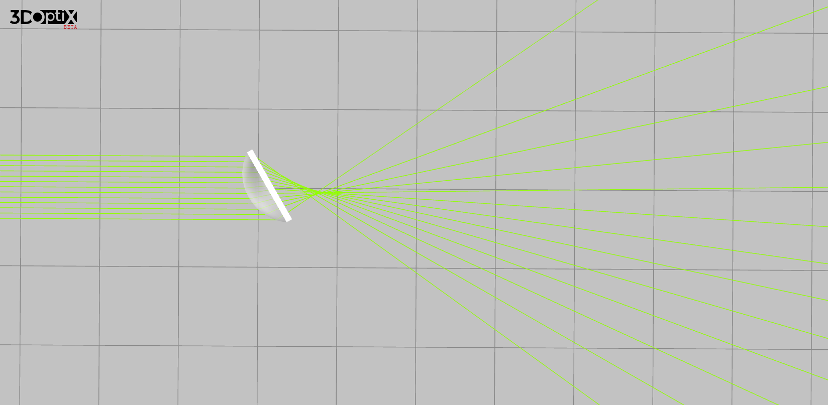
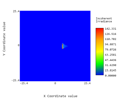
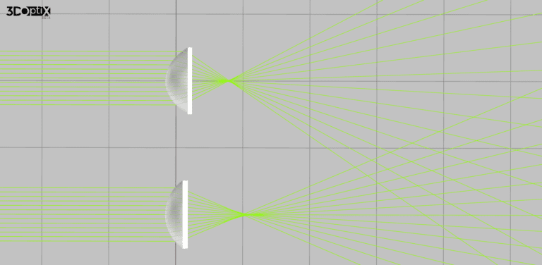
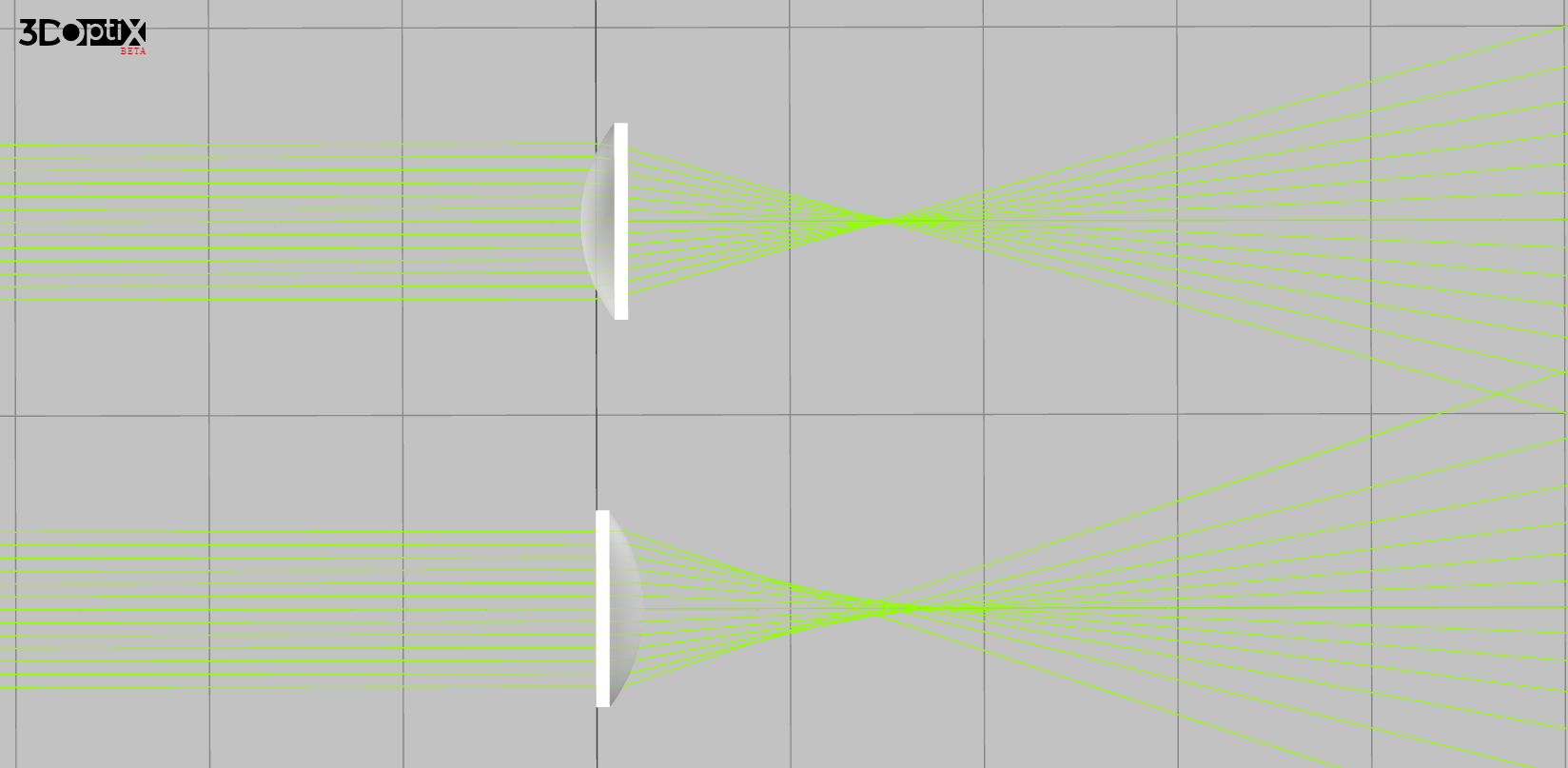
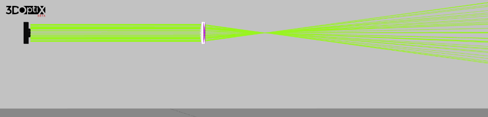
Fig. 7. Ray scheme and the PSF at different distances from a lens with astigmatism from two orientations. For the above (top) we see a shorter focal length than from the side (bottom). To simulate a lens with astigmatism, we combine two lenses, a cylindrical lens, and a regular lens.

Coma aberrations

Coma aberrations are the results of the z^3 term. Here, the imposed phase is no longer cylindrical symmetric so beams at the lower half of the lens will focus on a different location than beams at the upper half of the lens. Usually, this type of aberration happens when the light is not fully orthogonal to the lens, as is the case when looking at a distant star that is not in the center of the field of view. These aberrations are illustrated in Fig 8 where we present the focal length of a tilted lens with high coma aberration. At the image plane, we observe an asymmetric spot, which resembles a comet with a tail, which is the source for the name of these aberrations. In Fig 8 we present an image of a spot with high coma aberrations showing a coma-like trail.

Fig. 8. Coma aberrations due to tilted lens. (top) Ray tracing scheme. (bottom) Calculated measured spot.

There are several methods to overcome coma aberrations. All of them are based on compensating for the coma aberrations by a second optical element. The first way was invented by Bernhard Schmidt in 1930 and is called the Schmidt camera. In the Schmidt camera, we add a field flattener to the entrance of the telescope. This field flattener is a type of lens with a complex shape that compensates for the coma aberrations by introducing the opposite phase of the third-order coma aberrations. The second way was invented by Dmitry Dmitrievich Maksutov in 1941 and is based on adding a weak negative lens at the objective of the telescope. Then, we coat the central inner part of the lens with a reflective material so it becomes the secondary mirror. This method is idle when all the optical elements are spherical. However, spherical elements result in spherical aberrations, and therefore, most telescope resort to a hyperbolic primary mirror and a hyperbolic secondary mirror which are more complicated and expensive to fabricate but has a wider field of view than other telescopes. This method was invented by George Willis Ritchey together with Henri Chrétien in 1910. In this method, the main mirror has a positive curvature while the secondary mirror has a negative curvature. It compensates for all the aberrations when the radius of the main mirrors is:

R_1=-\frac{2DF}{F-B}=-\frac{2F}M

And the radius of the secondary mirror is:

R_2=-\frac{2DB}{F-B-D}=-\frac{2B}{M-1}

Where F is the effective focal length of the system, B is the back focal length namely, the distance from the secondary mirror to the focus, D is the distance between the two mirrors, and M = (F – B)/D is the secondary magnification.

To eliminate the spherical aberrations, we can resort to the Ritchey-Chretien telescope where the mirrors have the conic constants K_1 and K_2 and they are chosen according to:

K_1=-1-\frac{2B}{M^3D}

And 

K_2=-1-\frac2{{(M-1)}^3}(M(2M-1)+\frac BD)

Since both K_1 and K_2 are less than -1, the two mirrors are hyperbolic. 

Chromatic aberrations

Any glass has some dispersion which depends on the wavelength. Therefore, the index of refraction is a function of the wavelength, so the lens focal distance is also a function of the wavelength. This is illustrated in Fig. 9, where we see that the blue and the violet colors are focused at different focal distances. Usually, the index of refraction as a function of wavelength is 10^{-4}, which starts to affect imaging when we either image with broadband light or when the focal length is short and the lens is thick, so the influence of the dispersion is high.

Fig. 9. Shows that two different colors (red vs violet) are focused at different distances.

To overcome the chromatic aberrations in a telescope, we can replace the lens with a mirror. A mirror reflects all wavelengths in the same direction, and therefore, has no chromatic aberrations. In addition, it is possible to combine two lenses, each from a different type of glass, with the opposite chromatic aberration at the desired bandwidth, so their chromatic aberration cancels each other.

mascot-1-1

3DOptix works
only on desktop!

Please go to 3doptix.com on a
desktop device, using the
Chrome or Edge browser

Available on January 30th, 2023