Coherence and Interferometry

VIRTUAL LAB

Coherence and Interferometry

Course Overview
This laboratory course will introduce the student to the concept of coherence. A necessary understanding of the wave and particle nature of light will be reviewed for full comprehension of this concept. With an understanding of how these interactions occur, and the specific effects, simulation exercises will be conducted to build up concepts and optical systems in a reinforcing manner.
Course Duration

Approximately 3 hours (self-paced)

Learning Objectives
By the end of this pre-lab assignment, students should be able to:
  • Understand how light behaves as a wave
  • Describe the concept of coherence
  • Explain specific coherence effects
  • Construct various interferometers and analyze the output
Course Outline - Introduction to Coherence
Coherence is a fundamental concept in physics that describes the stability and consistency of waves. It refers to the degree to which waves maintain a constant phase relationship over time, space, or frequency. Coherent waves exhibit well-defined interference patterns when they overlap, allowing for precise measurements and analysis in various fields such as optics, telecommunications, and medical imaging. Maximizing coherence is essential in applications such as interferometry to ensure clear and accurate results. Overall, coherence plays a crucial role in understanding and harnessing the behavior of waves in diverse scientific and technological contexts.

Using a detector or a camera one can infer that diffraction or interference is happening due to the pattern created by the incident light. This pattern is described by light hitting the detecting device with high probability at one location and a lower probability at the other. This is known as constructive and destructive interference, which results in the well-known fringe pattern.

Interferometers leverage the coherence of waves to produce precise measurements and analysis. By combining coherent waves, interferometers create interference patterns that reveal information about the waves’ properties.
Coherence ensures that waves maintain a stable phase relationship, leading to well-defined interference patterns. Interferometers exploit this to detect small changes, enabling applications such as distance measurement, spectroscopy, and imaging with high accuracy and sensitivity. In essence, the coherent nature of waves is essential for the functioning of interferometers, allowing them to extract detailed information from the interference patterns they generate.

Light Waves and Coherence

Light acts (can be described) as a particle or wave depending on the specific experiment or phenomena being observed. This is the basis for the duality of light. In geometric optics, light is described as rays that take a straight path from surface to surface. Using this method, we assume that apertures are quite large compared to the wavelength of light and ignore effects such as diffraction. However, interference effects in that regime can be faithfully described using geometrical optics, if the rays carry both the amplitude and phase of waves.
Fig. 1. Rays traced through an optical system. The rays take straight line paths through both optical media and air. The apertures (optics) through which the rays pass are magnitudes larger than the wavelength of light.
Fig. 2. Left: Spherical wavefront generated from a point source. The wavefront expands in all directions. Right: Ray representation of the spherical wavefront. The rays (red) point along the wavefront and an infinite number of rays can be traced to reproduce a wavefront.
The wave nature of light can be thought of as a spherical wavefront propagating through a medium (such as air or the vacuum of space) in three dimensions. As the wavefront encounters different media (optical surfaces), the wavefront will distort, and if the aperture is very small, it will be diffract.

However, when two light waves impinge on the same surface and there exists a phase relationship between them that is not random, an interference pattern can be observed. This is the basis for interferometry. This measurement can give information about a sample’s composition, light source spectral composition, light source collimation, and optical component characteristics such as surface flatness.
Fig. 3. Two source points (purple dots) create spherical waves (blue and green circles). Where the waves intersect (red lines) constructive interference is observed. In between these points destructive interference is observed.
Experiment 1

Interferometers

There are many types of interferometers that are used for various applications. Regardless of the type, interference between one or more beams is used to determine the characteristics of the object under test. A few examples will be analyzed to determine the differences and how they operate. The Michelson interferometer is a very well-known instrument used for measuring optical component properties. One such property that can be measured is the wavelength of light sources. Using equation 1 below and counting fringes that traverse across a detector when moving a mirror, the wavelength of the source can be experimentally obtained.
1. \lambda = \frac{2d}{m}, where \lambda is the light source wavelength, d is the mirror displacement, and m is the number of times the fringe pattern repeats.
Care must be taken in a simulation environment that small steps, smaller than the wavelength under evaluation, are taken to ensure the fringes don’t move drastically and appear as a small shift. In a real laboratory experiment the fringes are easily seen to move across the detector when a mirror is rotated. If the wavelength of the source under evaluation is truly unknown it is best to start with a very small step size and move up from there to ensure accurate results. In a Mach Zehnder interferometer measuring wedge angles and surface flatness can be accomplished by inserting an optical element in the transmitted beam path and, similar to the Michelson interferometer, counting the fringes. Using equation 3 below, the wedge angle can be measured. For this measurement we do not need to move any optics in the interferometer, so this is a simpler technique.
2. \alpha = \frac{\lambda}{(n-1)S}, where \alpha is the wedge angle, \lambda is the light source wavelength, n is the index of refraction, and S is the fringe spacing.
A shear-plate interferometer is a useful and simple interferometric device for determining the collimation or divergence of a light source. Based on the fringe pattern angle from a reference axis one can tell if the beam is collimated or converging/diverging.
Exercise 1: Michelson Interferometer
  • The system is set up to measure the wavelength of the light source being used. The moving mirror will be moved to change the path length the light travels from the reflected path.
  • The wavelength of light is specified for the light source as 550 nm.
  • There is a reference detector that is locked to maintain the fringe pattern for a baseline comparison as the mirror is moved.
  • Click on the analysis displays for both detectors to bring them into their own window.  Then click in the center of the image to bring up the cross-section view for each.
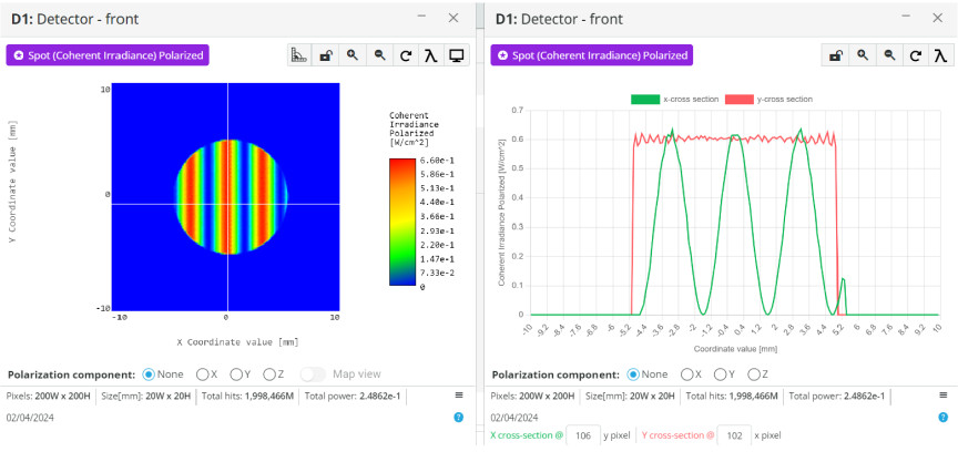
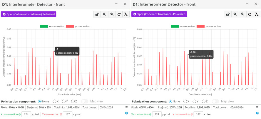
  • Using the cross section and the image of the two interference patterns, count the number of times the pattern repeats as the moving mirror is shifted towards the beam splitter 
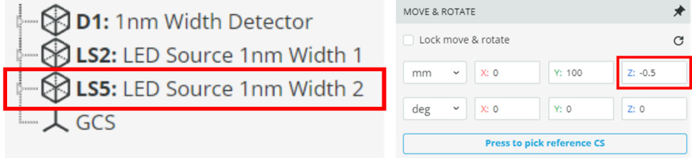
That is, reduce the “z” position of the moving mirror
  • Move the moving mirror towards the beam splitter (BS1) and count the number of fringes that pass a reference position. This is the number of the “repeated” pattern. The movement must be small enough so that the fringes can be seen moving from one side to the other of the analysis window. Try smaller nanometer movements until you can clearly see the fringes move.
  • The image below should be the setup for performing the measurement. Ensure the x-cross section and y-cross section are at the same pixel for both analysis windows.
  • Fill out the table below and calculate the wavelength. Clearly, we knew beforehand what the wavelength was and how small must be the steps to take, but the procedure is sound for testing unknown sources.
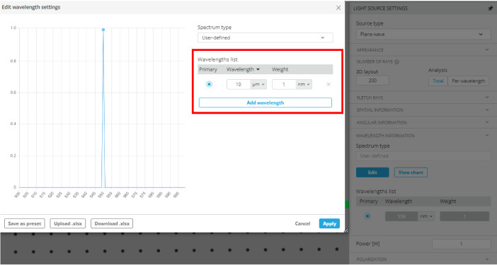
  • Change the light source wavelength to 10\mu{m} and repeat this procedure to calculate the source wavelength Notice you now need to use larger steps sizes to shift the fringesNotice that when the pattern is repeated for the first time (m=1) that the distance must be a specific value.  See equation 2 to understand what this distance must be.
The source wavelength can be measured very accurately using this method. Notice that the longer wavelengths are much easier to measure as the mirror is moved larger distances (microns versus nanometers) since the step size is related to the wavelength of the light source under test. In real world optical systems nanometer accuracy is not practical and using this method is only feasible for the longer wavelengths.
Extra information
The Michelson interferometer was invented by the American physicist Albert A. Michelson in the late 19th century. Michelson devised this optical instrument in 1881 to measure the speed of light more accurately. His motivation stemmed from the belief that precise measurements of light’s velocity could provide insight into fundamental physics and improve scientific understanding.
The interferometer proved to be a versatile tool beyond its original purpose, facilitating groundbreaking experiments in fields such as spectroscopy, astronomy, and metrology. Michelson’s invention significantly contributed to the advancement of physics and remains a cornerstone of optical instrumentation and experimental techniques.
The Michelson-Morley interferometer, devised in 1887 by Albert A. Michelson and Edward W. Morley, aimed to detect the existence of the luminiferous aether, a hypothetical medium thought to permeate space through which light waves were believed to propagate.
According to the prevailing theory at the time, earth’s movement through the aether should have caused a detectable difference in the speed of light along these paths, leading to a measurable interference pattern. However, the experiment yielded a null result, showing no significant difference in the speed of light along the two paths.
This unexpected outcome challenged the notion of the luminiferous aether and provided crucial evidence supporting Albert Einstein’s later theory of special relativity, which posits that the speed of light is constant in all inertial frames of reference. The Michelson-Morley interferometer thus played a pivotal role in revolutionizing our understanding of space, time, and the nature of light.
Exercise 2: Mach Zender Interferometer
  • The system is set up to measure the wedge angle of a flat optic such as a wedged window.
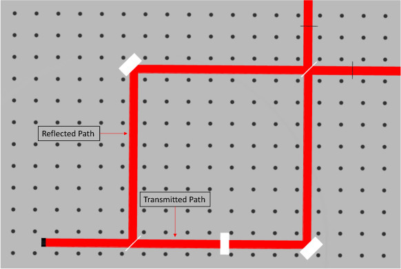
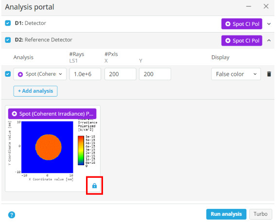
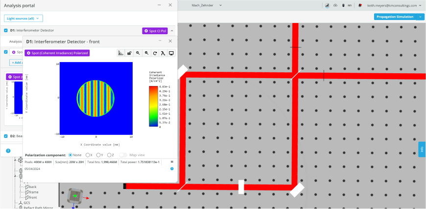
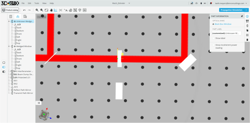
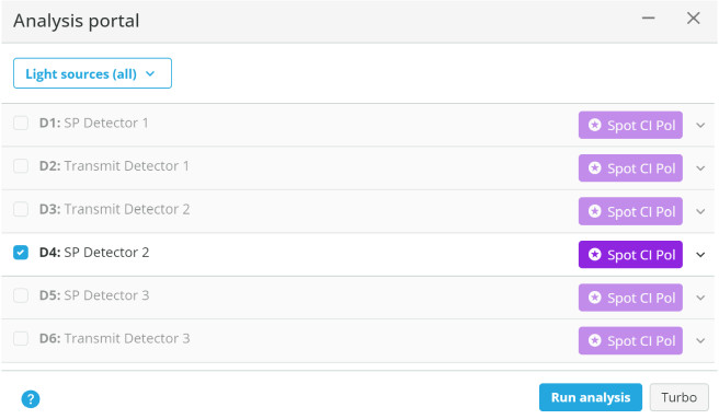
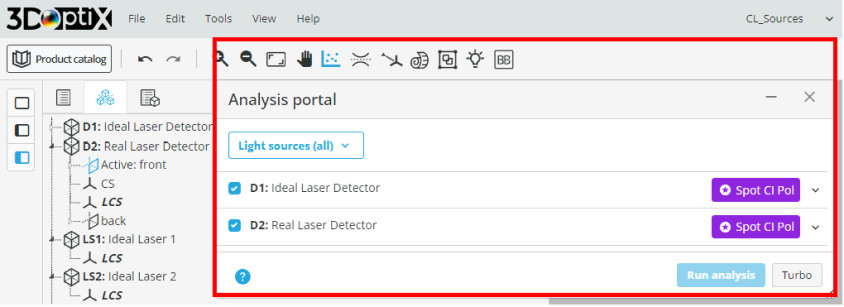
  • First open the analysis portal and run analysis to generate the baseline interference pattern. 
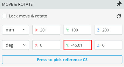
Note that BS2 is tilted 0.01 degrees to increase the fringe frequency.
  • Now click on the flat optics to the right of BS1 and change the wedge angle to 0.5 degrees.
  • Since the wedge angle will increase the fringe frequency we want to remove BS2’s tilt.  Change the Y-angle to 45 degrees from the original 45.01 degrees.
  • Run analysis and click on the detector window. Click in the center of the interference pattern to bring up the cross-section view.
  • By zooming in on the graph and moving your cursor over the peak, the distance between two peaks can be measured.
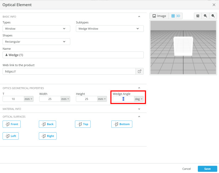
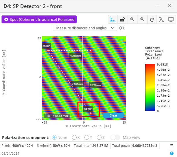
  • Fill in the table below using equation 2 for the above result and four more measurements to get an average value of the wedge angle. Remember to multiply the value for the wedge angle you calculate by 180/pi to get the angle in degrees.
  • There is another optics named unknown wedged window in the 3D layout.  Move this window into the position of the window just measured.
  • Repeat the method previously used and calculate the wedge angle using five different points in the interference pattern. 
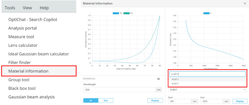
The material of the unknown window is N-SF11. Use the materials tool to determine what the index of refraction is.
  • Look at the wedge angle when you are finished with the calculations.
Precise measurements of wedge angle can be made with this technique. Notice that the results are very close due to the exact nature of the simulation software. This is a good first check if results from experiments are difficult to approximate or fringe contrast is low.
Notice that the wedge angle must be below some threshold or else the light will be angled out of the optical system. For higher wedge angles the optical path length of the interferometer can be shortened to allow for a measurement.
Extra information
The Mach-Zehnder interferometer is named after its inventors, Ludwig Mach and Ludwig Zehnder, who developed it independently of each other in the early 20th century.
Ludwig Mach, an Austrian physicist, first described the basic principle of the interferometer in 1891. He proposed an interferometric setup that split a light beam into two paths using a half-silvered mirror (beam splitter), directing them through different optical paths before recombining them to produce interference fringes. However, Mach’s design wasn’t practical at the time due to limitations in technology.
Around the same time, Ludwig Zehnder, a Swiss physicist, developed a similar interferometer in 1891, independently of Mach’s work. Zehnder’s design was more practical and consisted of a light source, a beam splitter, mirrors, and a viewing screen. This setup allowed for the interference pattern to be easily observed and analyzed.
It wasn’t until the mid-20th century that the Mach-Zehnder interferometer gained widespread recognition and became a crucial tool in optics, quantum mechanics, and various other scientific disciplines. Its sensitivity and versatility have made it an indispensable instrument for measuring small changes in phase, amplitude, and optical properties of materials.
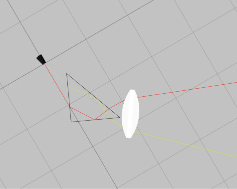
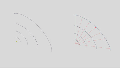
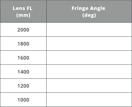
Exercise 3: Shear-Plate Interferometer
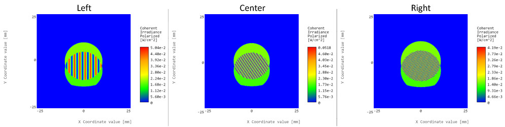
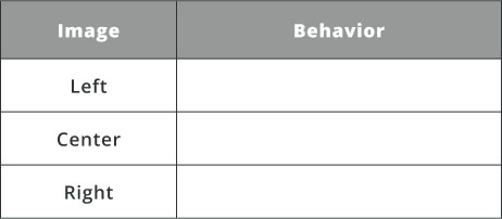
  • Before doing any analysis in the simulation file, fill in the table with a guess as to the light behavior based on the images below. The light source is either collimated, diverging, or converging.
  • Now open the analysis portal and run analysis to generate the interference patterns for the three optical systems.  Check each shear-plate interferometer detector and lens configuration to see if your guesses were correct.
  • Deselect all detectors except for SP Detector 2.
  • Determine the angle that the fringes make with respect to the y-axis of the detector. Use the measure mode tool to do this by making a right-angle triangle with the hypotenuse following a fringe.
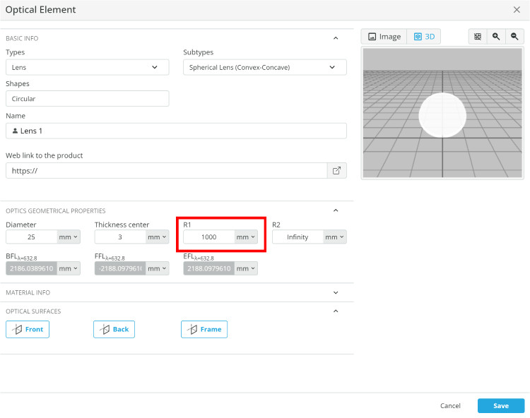
  • Change the focal length by changing the radius of curvature (R1) of lens 1 to the values in the table and record what the fringe angles are, using the method above. The values do not need to be perfect for the focal length. Using an integer value for R1 will be sufficient. Increase the pixel count if the fringe pattern is not visible.
  • Graph the values using excel or a plotting program with the x values the lens focal length and the y values the fringe angle.  Determine if the correlation is linear, polynomial, or another fit.
Extra information
Shear plate interferometers have their origins in the rich history of interferometry, tracing back to the foundational work of scientists like Albert A. Michelson in the late 19th century.
While Michelson’s interferometer laid the groundwork for precise measurements using interference patterns, further advancements were made in the early 20th century by physicists Frank Twyman and Stanley Green. Their innovation involved introducing a shear between interfering beams by utilizing a transparent wedge-shaped plate, known as a shear plate.
This development significantly enhanced the sensitivity and versatility of interferometric measurements, particularly in optical testing and metrology applications.
Over time, shear plate interferometers have undergone continuous refinement, benefiting from advancements in laser technology and becoming indispensable tools in fields such as precision engineering, semiconductor manufacturing, astronomy, and biomedical imaging, enabling highly precise and non-destructive measurements of small displacements, surface irregularities, and optical aberrations.

Temporal Coherence

The mean temporal coherence is directly correlated to the center wavelength and spectral bandwidth of the light source.
3. L_c=\frac{\lambda^2}{\Delta\lambda}, where \lambda is the light source wavelength, d is the mirror displacement, and \Delta\lambda is the spectral bandwidth.
As can be seen from equation 3, light sources such as lasers that can have spectral bandwidths in the picometer range will have an extremely long coherence length. On the other hand, LED’s with very large spectral bandwidths will have very short coherence lengths.
Experiment 2

Determining Coherence

The spectral characteristics of a source will dictate its coherence and a large range of values can be realized. Different coherence lengths are useful in different applications. Using equation 3 from above, the coherence length of sources can be compared. As specific applications typically only allow a certain wavelength range to be used (due to material properties), the spectral bandwidth will be the variable parameters.
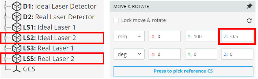
Exercise 4: Laser Coherence Length
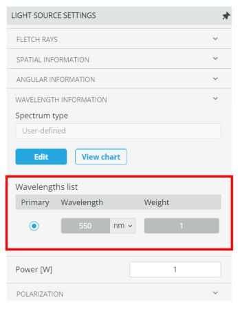
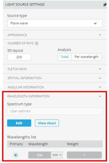
  • There is an ideal and a real laser source. Find the spectral bandwidth by clicking on each source and scrolling down to the wavelengths tab. The spectral bandwidth is the difference between the minimum and maximum wavelength.
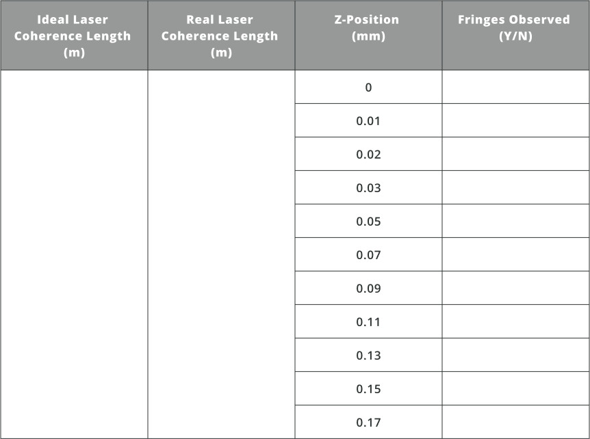
  • Calculate the coherence length for each source and fill in the values in the table below. As the ideal laser is perfectly monochromatic the coherence will be infinite, i.e. there is no spectral bandwidth.
  • Open the analysis portal and run analysis.
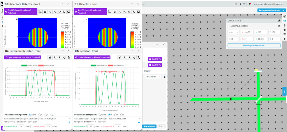
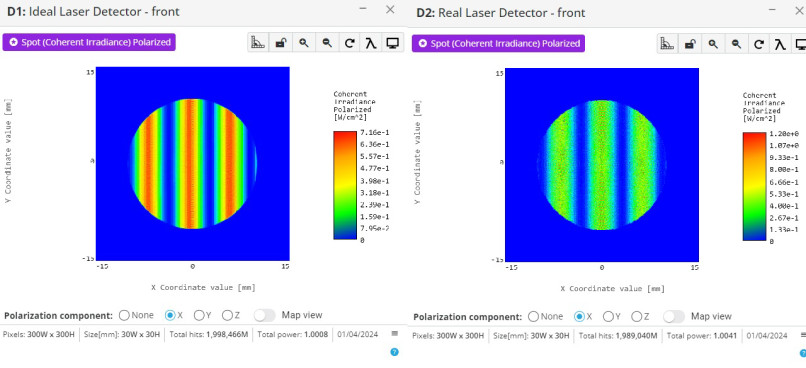
  • Observe the fringes for both analysis windows. Notice that the contrast between the ideal and real laser patterns are different.
  • Next, move the “2” sources to the positions in the table and record if fringes are observed.
No source is perfectly monochromatic, so the real laser used in this simulation is not realizable. However, it demonstrates that a perfectly monochromatic source would have infinite coherence length. This can be seen in the table above as the fringes in the real laser setup disappear after the coherence length has been reached, but the ideal laser will have fringes with the detector placed at any position.
Extra information
The origins of laser coherence lie in the principles of stimulated emission and optical feedback within the laser cavity. When atoms or molecules within a laser gain excess energy through an external source, they enter a metastable state. Stimulated emission occurs when a photon interacts with an atom or molecule in this excited state, causing it to emit another photon with the same frequency, phase, and direction as the incident photon. This process leads to the amplification of light waves, resulting in a coherent beam. Pulsed laser can have the ability to be completely coherent depending on the pulse width.
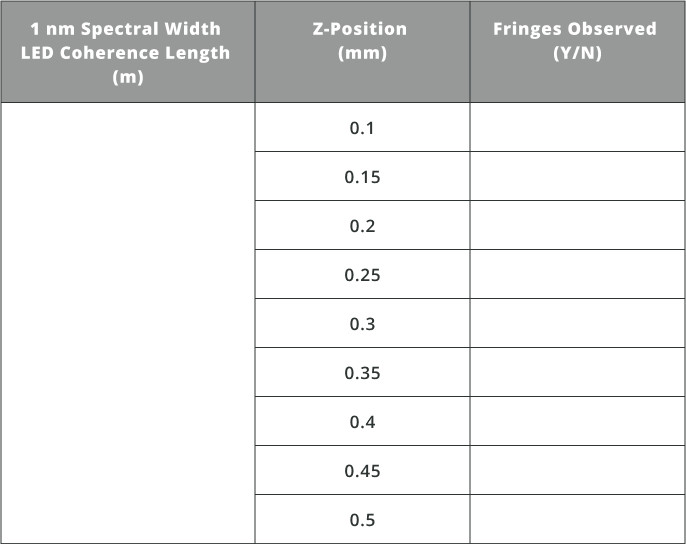
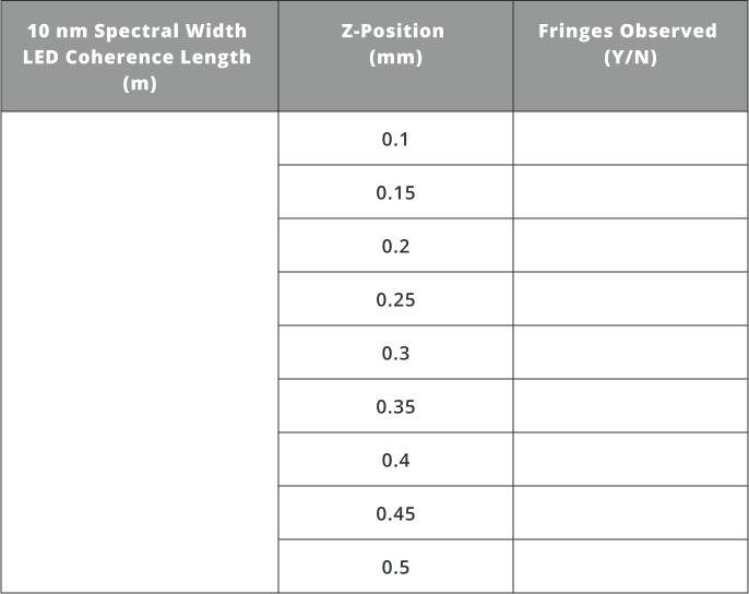
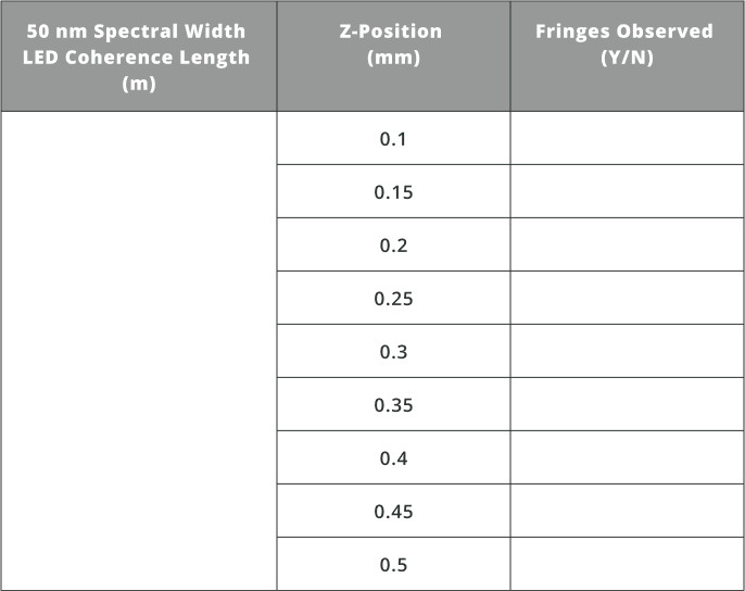
Exercise 5: LED Coherence Length
  • Import the file “CL_LED1.opt” into the 3DOptix app.
  • Calculate the coherence length and fill in the value in the table below.
  • Next, move the “2” source to the positions in the table and record if fringes are observed.
In comparison with the laser sources in exercise 4, the coherence length of LED’s is much shorter. Choosing an LED with a certain spectral bandwidth will change the coherence length as can be seen by the analysis above.
Extra information
LEDs with enhanced temporal coherence are finding applications in various fields where precise optical control is necessary. In fiber-optic communications, these LEDs enable higher data rates and longer transmission distances, offering cost-effective alternatives to laser-based systems. In medical imaging, such as optical coherence tomography, improved coherence enhances image quality and diagnostic capabilities.
Additionally, in interferometry, spectroscopy, and optical sensing, LEDs with controlled coherence provide accurate measurements with simplified setups compared to traditional laser sources.
In 3D scanning and imaging, these LEDs contribute to higher resolution and accuracy, benefiting applications in industrial inspection, robotics, and augmented reality. Overall, the development of LEDs with enhanced temporal coherence expands their utility across diverse domains, offering efficient and precise optical solutions.
Analysis and Conclusion
Coherence and interferometers are incredibly important concepts and optical tools that are indispensable in modern day physics and optics. Understanding the concept of coherence and how to utilize it opens up a variety of methods and techniques to create deterministic experiments for a variety of applications. This course has reviewed the fundamental properties of coherence and the exploitation of this concept to create interference patterns with interferometers.
Assessment
NA
Resources
The student requires an account in the 3DOptix system.
Synopsys
In this course, students immerse themselves in the wave phenomena of light and the application of coherence. The curriculum delves into the core principles of temporal coherence, interference, multi-source wave interactions, and applications in optical measurements. Through engaging experiments and exercises, students acquire a profound comprehension of these concepts and their pragmatic applications.
mascot-1-1

3DOptix works
only on desktop!

Please go to 3doptix.com on a
desktop device, using the
Chrome or Edge browser

Available on January 30th, 2023