

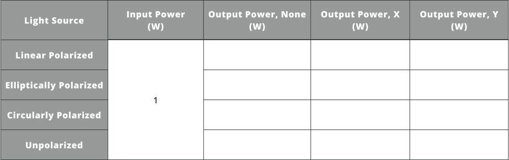
Exercise 1: Polarized Light Sources
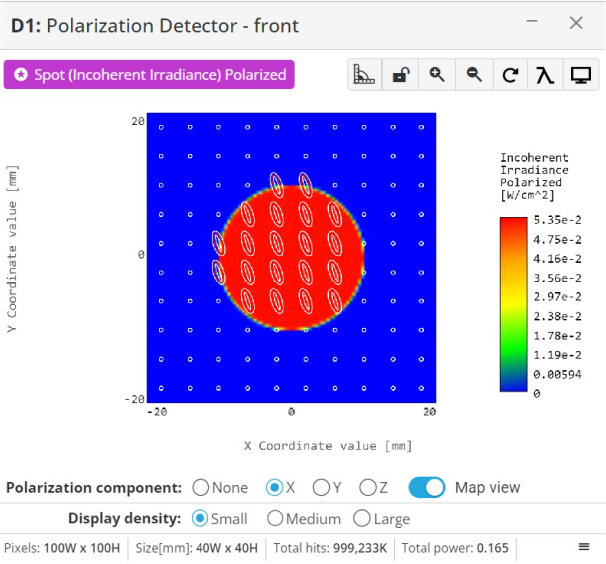
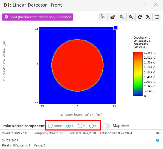
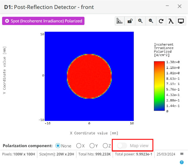
- Click on the analysis detector to bring it into its own window
 Notice on the bottom of the window there are four options to view the power for each polarization state; none, x, y, and z
- Select polarization state “None”, x, and y to see how much power is present for each
We are not interested in the z component as it is not present in these polarization states
- Record these values in the table below
The “None” option includes power for all polarization states
Exercise 2: Polarizer Optics
- Click on the analysis portal and select run analysis
There is a polarizer inserted into the optical path to change the amount of light that makes it to the detector. The extinction ratio is 60 dB, so very little light from the opposite polarization will make it through to the detector when aligned with the polarization axis of the light source.
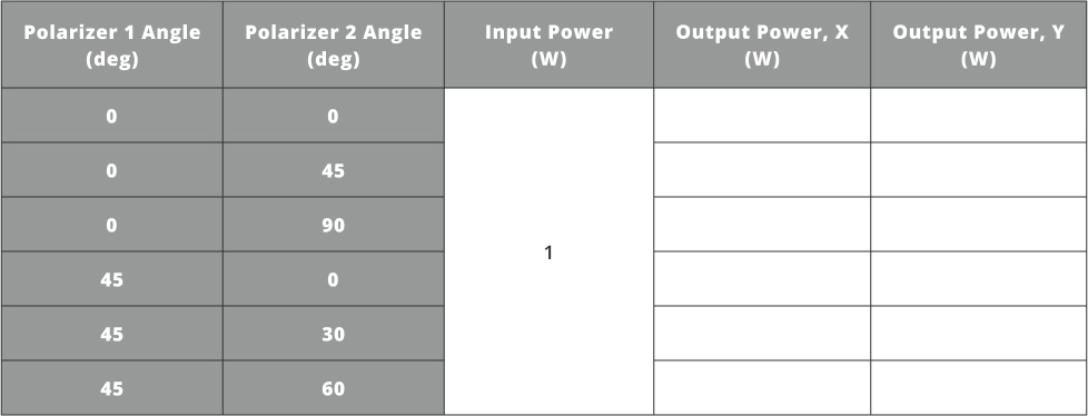
Exercise 3: Multiple Polarizers

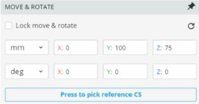
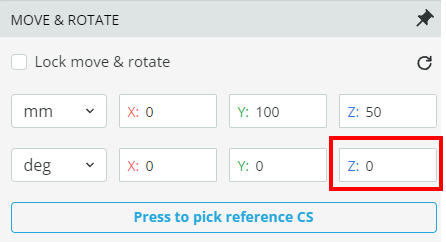
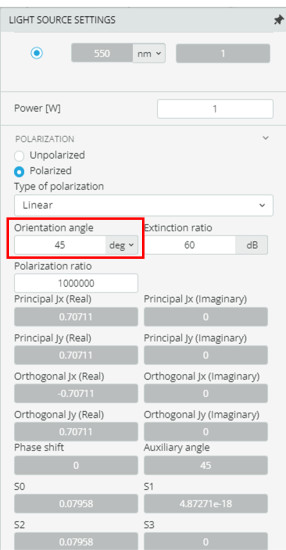
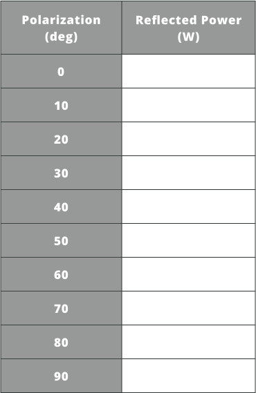
- Change the rotation angle to the values in the table below, run analysis, and record the power
Notice that there are locations of minimum and maximum transmission for both a single polarizer and dual polarizers
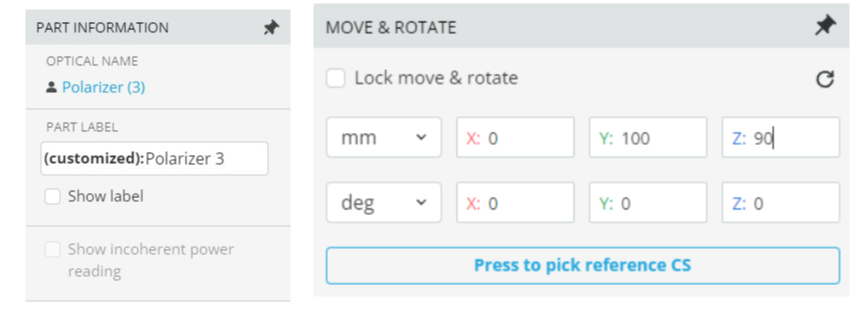
- Change polarizer 2 and 3 angle to z = 90
Polarizer 1 should be z = 0 degrees

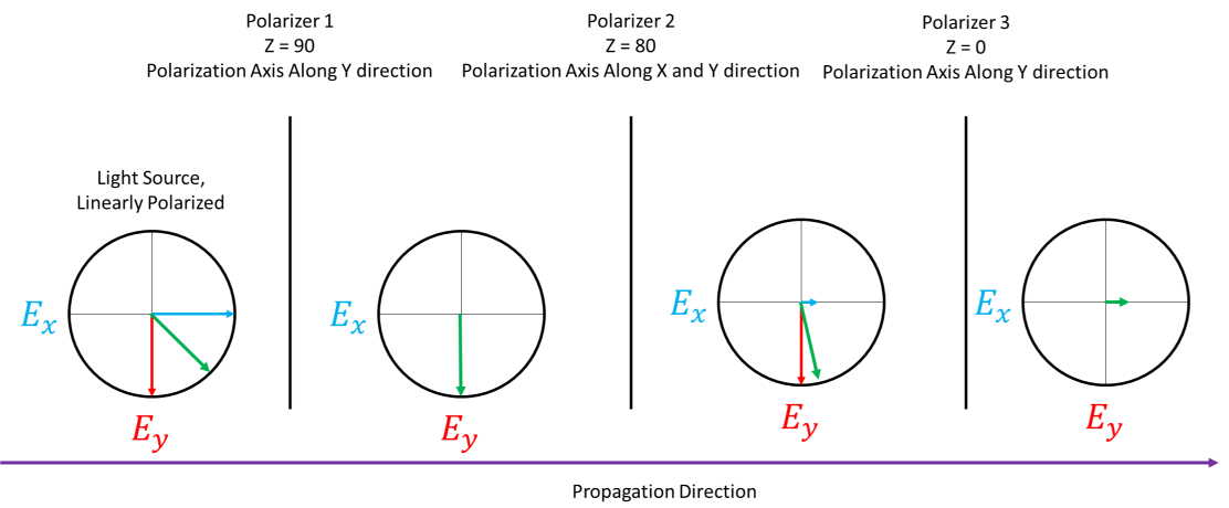
- Run analysis and observe the power on the detector for both “x” and “y” polarization states
We now have “crossed” polarizers, between polarizer 1 and 2/3, and should not see any transmission to the detector
- Run analysis and observe the power on the detector for both “x” and “y” polarization states
We still have crossed polarizers, between polarizer 1 and 2, and should not observe any power still on the detector
- Run analysis and observe the power on the detector for both “x” and “y” polarization states
We now have light on the detector even though polarizers 1 and 3 are crossed. This is contradictory.
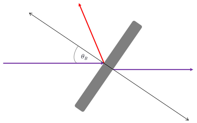
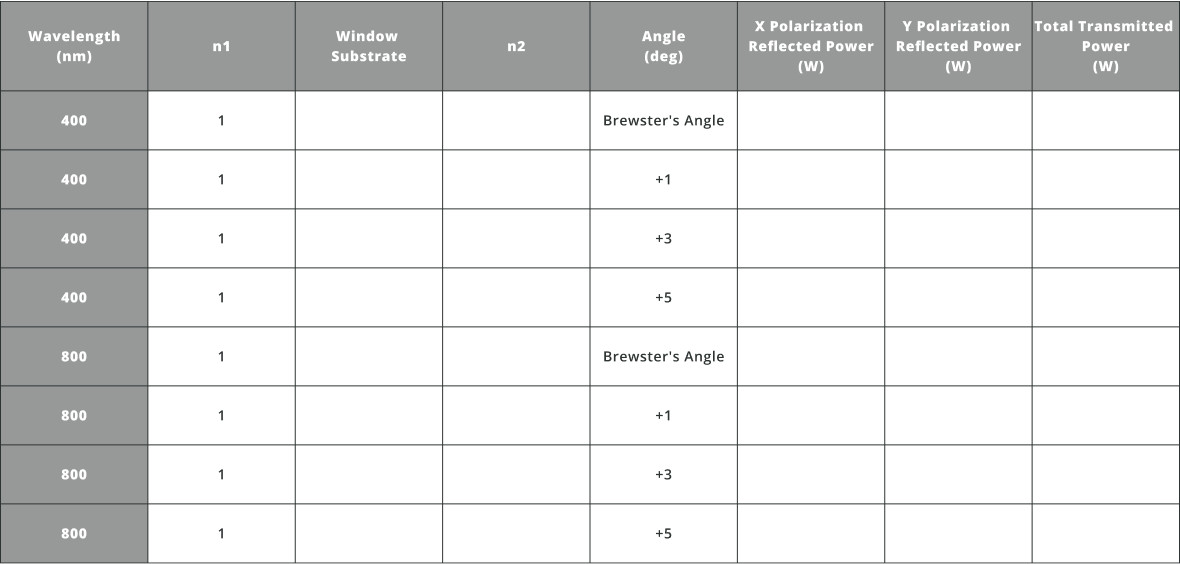
Exercise 4: Brewster’s Angle
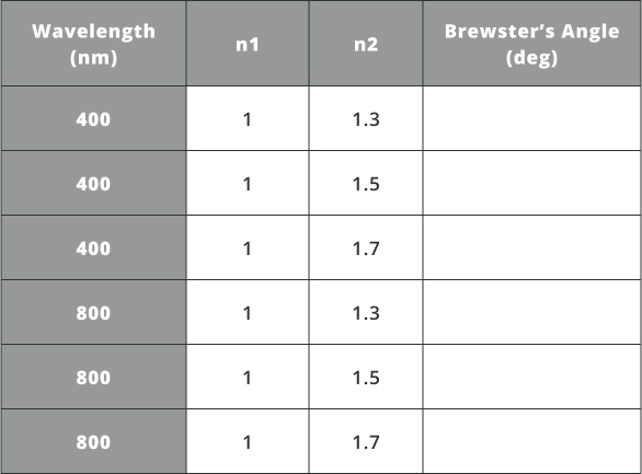
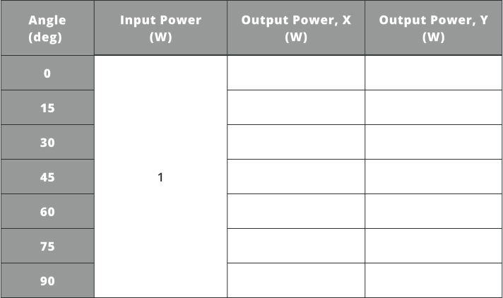
- Fill in the table below for the substrate used, index of refraction of the medium, and reflected and transmitted power at the specified angles
The offset angles are displaced from Brewster’s angle, e.g. if Brewster’s angle is 56 degrees and the angle is +1, then the angle of the Brewster’s window would be 57 degrees

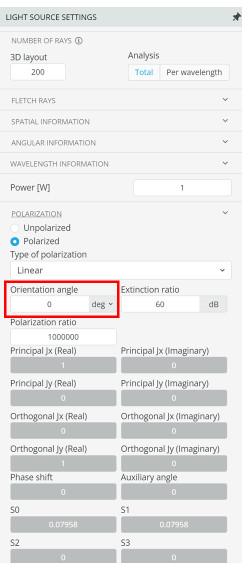
- Now change the light source polarization to 90 degrees corresponding to a vertically polarized linear state and fill out the same table with the new polarization state
Notice that this polarization state does not exhibit the same behavior as the other state
Exercise 5: Beam Sampler
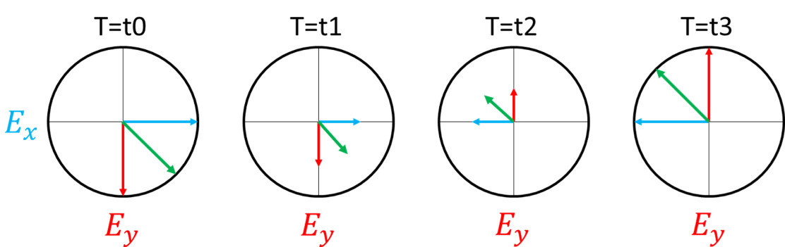
Exercise 6: Circular Polarized Light
- Using equation 3, calculate the parameters needed to create a quarter waveplate to circularly polarize a linear light source at 660 nm
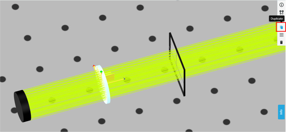
Use the user defined object that is in the 3D layout

- If the quarter waveplate was implemented correctly, the map view will show circular polarization over the spatial intensity field
The polarization state will not be perfect, but should look somewhat elliptical and close to circularTry 1.301365 and 1.31 for the two indices and 12.7 mm for the thickness if other values are not working