Spectroscopy

VIRTUAL LAB

Spectroscopy

Course Overview
This pre-lab assignment aims to introduce students to spectroscopy and its fundamental principles. Students will create different types of spectrometers and analyze the spectrum generated by the radiating source. During the analysis phase, students will gain a deep understanding not only of design challenges but also the theoretical backgrounds. The course will cover reflection and transmission gratings inside of the diffraction spectrometer, along with the specific analysis required to evaluate the designed spectrometer.
Course Duration
Approximately 3 hours (self-paced)
Learning Objectives
By the end of this pre-lab assignment, students should be able to:
  • Understand the basic principles of Spectroscopy
  • Comprehend diffraction gratings (Reflective and Transmissive) and diffraction by grating
  • Explore Spectrometers or Spectrographs and Monochromators
  • Analyze the various sources’ spectra using a diffraction spectrometer
  • Understand diffraction spectrometer theory using a simulation setup
Course Outline - Introduction to Spectroscopy:
Spectroscopy is a scientific discipline that involves the study of electromagnetic radiation spectra using spectroscopic equipment. These systems analyze radiation by dividing it into spectral components. Since light exhibits electromagnetic wave properties, we can separate its electromagnetic components and analyze each one. This is achieved using optical components such as prisms and gratings, and various spectroscopic instruments are used to analyze these components. The types of systems mentioned below are listed in the table. For this lab, we will focus on the fundamental designs of a spectrometer and a monochromator.

Basic Principles of Spectroscopy

System Type
Principle
Spectroscope
Inspecting the spectral content through visual observation
Spectrometer
Measuring the spatial or angular deviation in a dispersing system to determine the spectral distribution of a radiation under test
Monochromator
Only the part of the radiation that corresponds to a small spectroscopic component is detected after it has been separated
Spectrograph
Utilization of sensor for the detection of complete spectrum
Spectral photometer
A type of monochromator that is equipped with a sensitive detector
To analyze the radiating spectrum, a spectrometer utilizes either a dispersing or a diffracting optical element to distribute light into its spectral components. This can be achieved using either a prism or a grating. A collimating lens is employed to collimate the diverging light source, which is then focused onto the entrance slit. If a prism is used for analysis, dispersion occurs, dispersing light at different angles. With grating, the light is diffracted into various diffraction orders. Subsequently, the light is focused to convert angular separation into spatial separation at the exit slit, where a small spectral segment falls onto the detector.
When only a specific part of the spectrum is of interest and is filtered by the exit slit or an absorption filter, this configuration is termed a monochromator. Spectrometer performance criteria include spectral resolution and sensitivity to small energies, which define the system’s étendue and effective dispersion. Étendue represents the system’s throughput or the amount of light it accepts. Generally, higher spectrometer resolution correlates with lower étendue. Étendue is determined by the following equation
G = A\Omega
where \Omega is the solid angle of the source and A is the area of the slit
The étendue for slower optics (f/# < f/5) can be approximated to:
G = \frac{SA_s}{p^2}=\frac{S^{\prime}A_{slit}}{q^2} where p and q are the object and image distance, A_s and A_{slit} are the areas of the source and slit, S and S^{\prime} are the area of source and entrance slit \Omega = \frac{A_s}{p^2}
The best throughput is achieved by optimizing the light source that is imaged onto the entrance slit so that the solid angle of the incoming light matches the acceptance angle of the spectrometer. This approach also helps to avoid scattering within the system.
The spectral resolution of a spectrometer defines its ability to resolve fine wavelengths, specifically the smallest distance between two spectral peaks at which they can be distinguished. The spectral resolution is determined by the following equation:
SR = \frac{\lambda}{d\lambda} = mN
where \lambda is the measured wavelength and the d\lambda is the full width half maximum (FWHM) of the measured spectral peak (wavelength). N is the number of groves illuminated and m is the diffraction order.
The factors which affect the resolution are:
  • Slit width
  • Diffraction grating
  • Detector pixel array density
Increasing the slit width spacing decreases the resolution, whereas increasing the number of gratings per mm and the pixel density will improve the resolution. Finally, the spectral bandwidth of a spectrometer defines the range of wavelengths that the spectrometer (detector) can detect, and it is defined by the following equation:
\Delta\lambda = \frac{\Lambda}{fd}
where d is the detector size, f is the focal length of the lens and \Lambda is the periodicity of the grating.
Spectroscopic instruments are essential tools for identifying substances, measuring concentrations, and exploring molecular interactions using methods such as absorption, transmission, and emission. Now that the basic principles of spectrometry have been discussed, let us proceed to construct a few spectrometers and analyze them in greater detail.
Experiment 1

Building Czerny-Turner Spectrometer

A Czerny-Turner spectrometer consists of an entrance slit, an exit slit, a reflective diffraction grating, and mirrors. The objective is to take a broadband source, divide its components, and extract a single spectral wavelength. As we proceed, we will investigate the behavior of each component and document our observations. We will start by defining and analyzing each component step by step.
Exercise 1: Defining Broadband source
  • Import the file “Ex_1_CT_Spectrometer_LS.opt” into the 3DOptix app.
  • As shown below, the system at this point contains only a light source and a detector.
  • The next step is to choose the light source and edit the wavelength information. Define the wavelength range of the source with a Top-Hat profile. This is done by the following method:
  • Once a light source is selected, a ribbon will appear on the right-hand side. Go to the source setting by clicking the Light source settings.
  • Expand the Wavelength information and click the edit button to edit the wavelength information and define the spectrum.
  • Select the spectrum type as TH, specify the wavelengths as shown below and click Apply.
  • The result of the source definition is shown below. In this way, we have defined our broadband (polychromatic) source.
  • Before running the analysis, change the layout rays based on the defined wavelengths. Go to the toolbar and under View, change the “Change ray color palette” to Spectral ray colors. This will help us later to analyze each wavelength separately.
  • Open the Analysis portal and click Run analysis. The settings are shown below.
  • Click on the Detector window to enlarge the window.
  • Click on the top right corner on the Display type and select Spectral view.
  • Notice the output. The source is displayed as white. This is because we have defined multiple wavelengths that constitute our broadband source.
  • Switch back to False color mode and record the Total power and the power of each wavelength. The wavelengths can be filtered by using the option shown below (you can choose which wavelength to keep in the analysis window).
Hint: Since the source profile is Top-Hat (TH), each wavelength has the same weight.
Extra information
In the early development of spectroscopy, Isaac Newton’s experiments in 1666 demonstrated that white light is composed of a spectrum of colors, achieved by passing sunlight through a prism, thus laying the foundational understanding of light. Later, in 1814, Joseph von Fraunhofer discovered dark lines in the solar spectrum, now known as Fraunhofer lines, which indicated that specific wavelengths were absorbed by elements in the sun’s atmosphere. These discoveries were crucial in establishing the principles of spectroscopy. Significant advancements in spectroscopy occurred during the 19th century. Between 1859 and 1860, Gustav Kirchhoff and Robert Bunsen established the principles of spectroscopy, showing that each chemical element generates a unique spectrum of lines in both emission and absorption. In 1864, James Clerk Maxwell’s development of the theory of electromagnetism provided a theoretical basis for understanding light as an electromagnetic wave. In 1868, William Huggins further advanced the field by applying spectroscopy to astronomy, identifying chemical elements in stars and nebulae, thereby initiating the era of astrophysical spectroscopy.
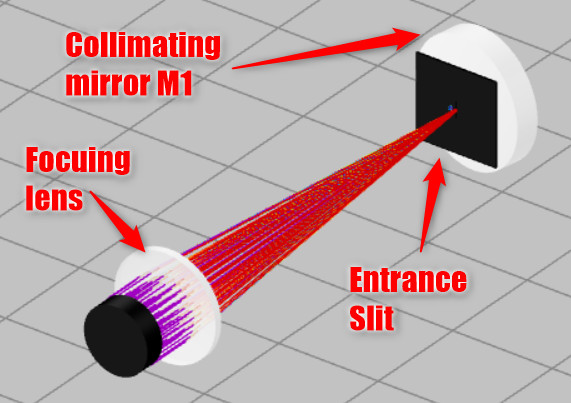
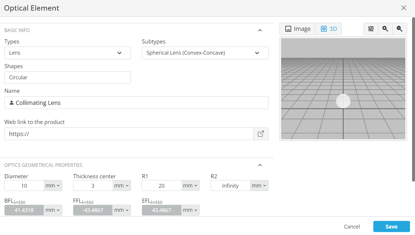
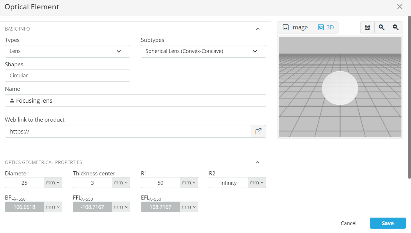
Exercise 2: Selecting a focusing lens, entrance slit and Collimating Mirror
  • The goal is to have a high throughput by collecting all the light at Mirror M1 and to collimate it.
  • Open the Optical properties of the focusing lens. Record the back focal length (BFL). This is done by right-clicking on the lens and then opening the optical settings of the lens.
  • Change the distance (Z) between the lens and the Mirror M1 such that the light is collimated without any loss of the incident light at the Mirror M1.
  • Hint: This is achieved by matching the angle of the incoming light with the acceptance angle of the Mirror M1.
  • Observe the detector output by opening the Analysis portal and clicking Run analysis.
  • What do you see?
  • Now calculate the etendue or the throughput of the system using the equation mentioned above. Keep the height of the entrance slit the same.
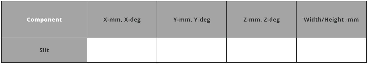
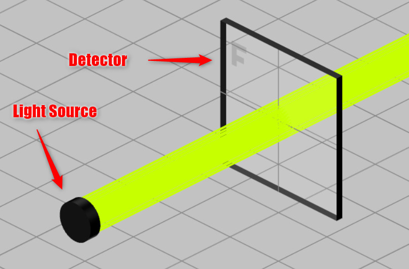
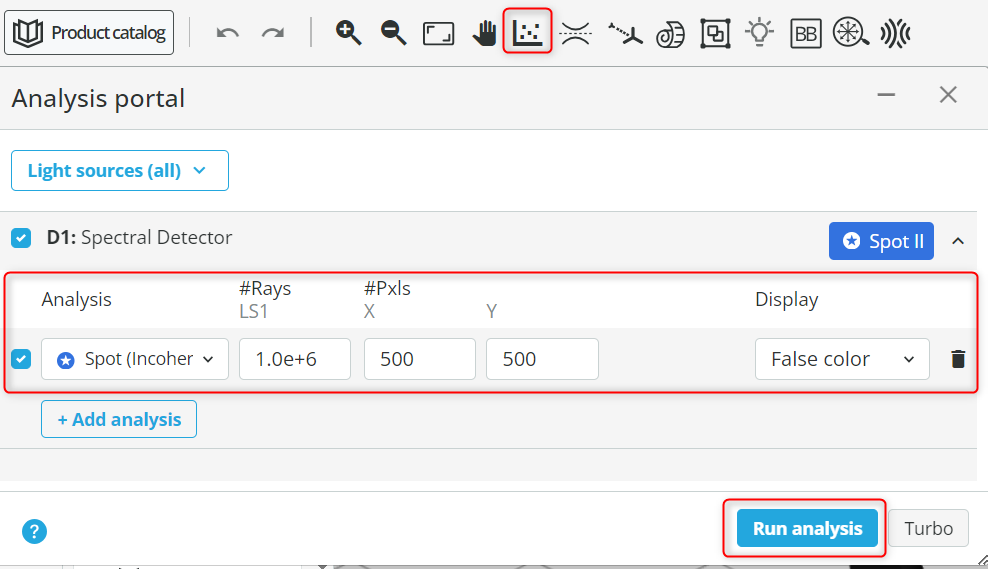
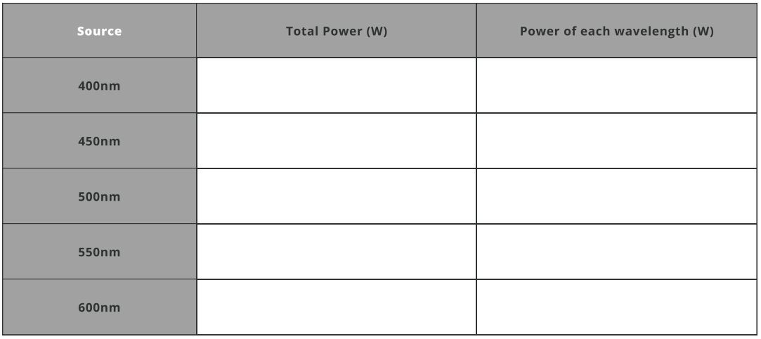
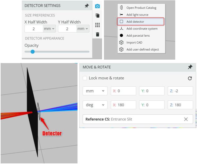
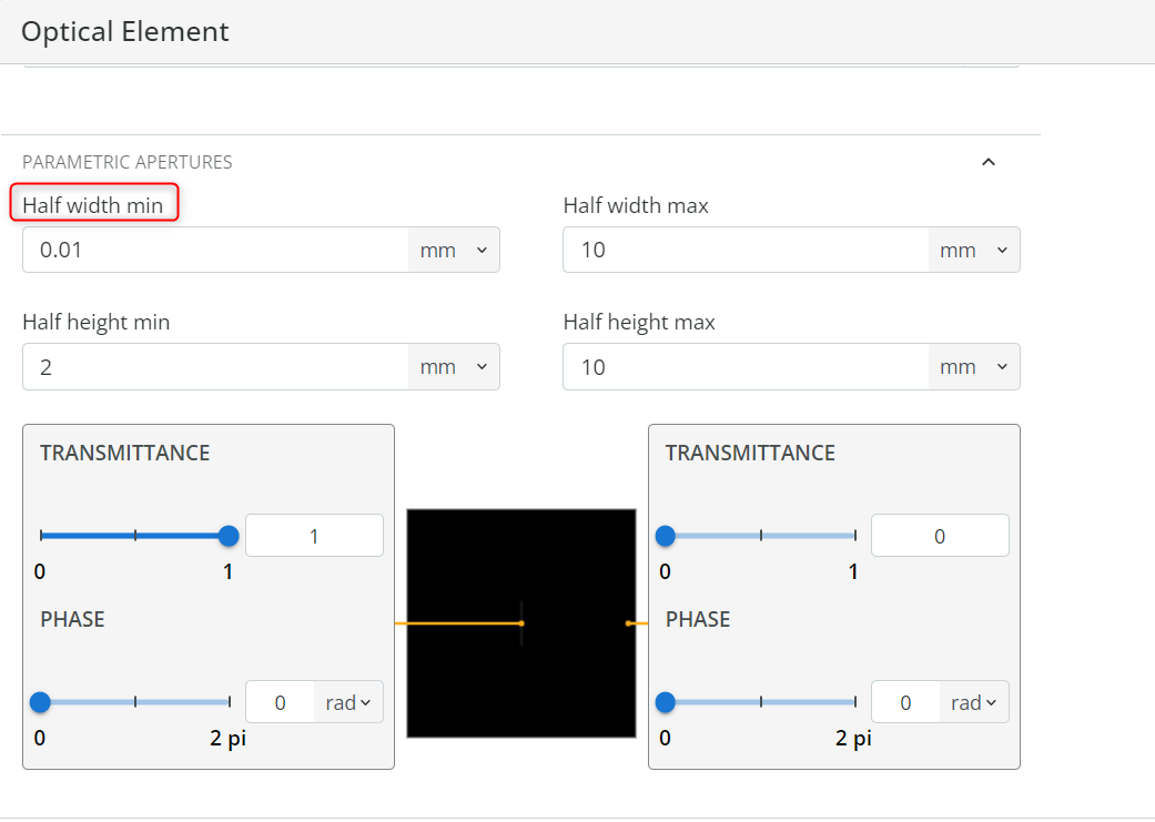
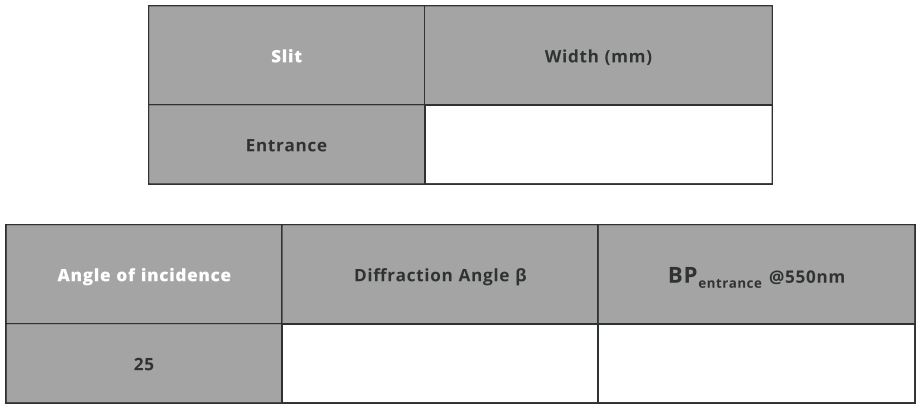
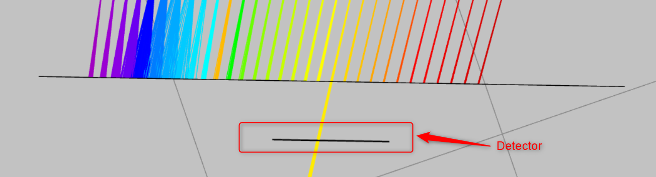
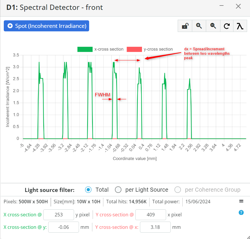
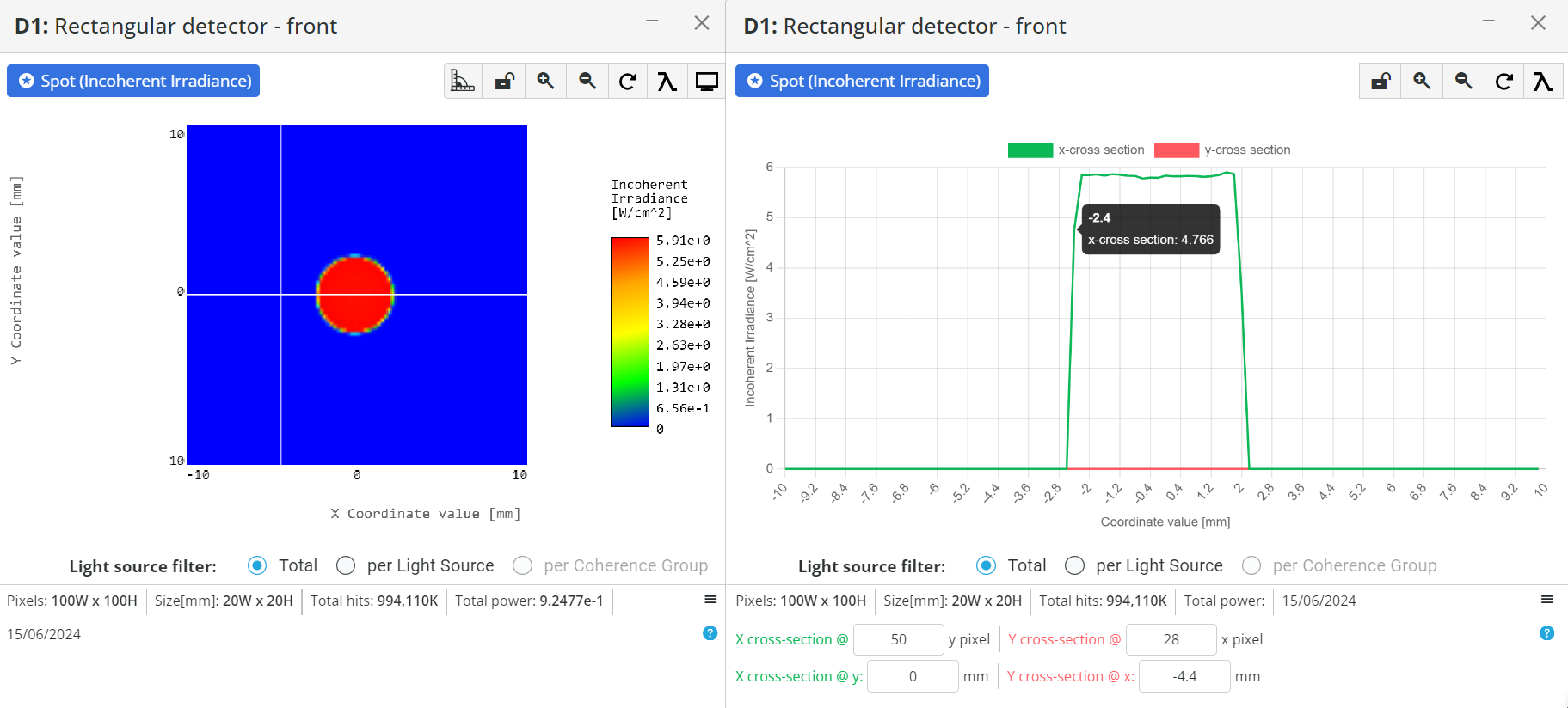
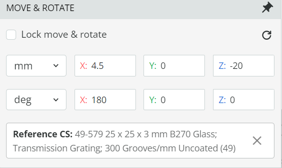
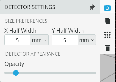
  • Place the detector after the entrance slit at 2mm, as shown below, and record the total power of the whole spectrum and the total power of the mentioned wavelengths. The half-width and height of the detector is 5mm and is referenced to the entrance slit. 
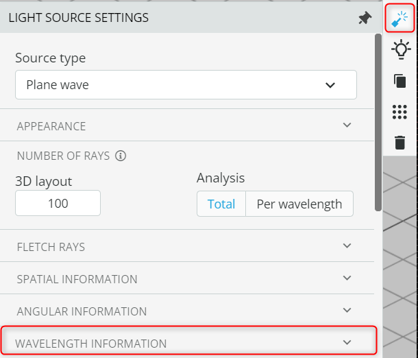
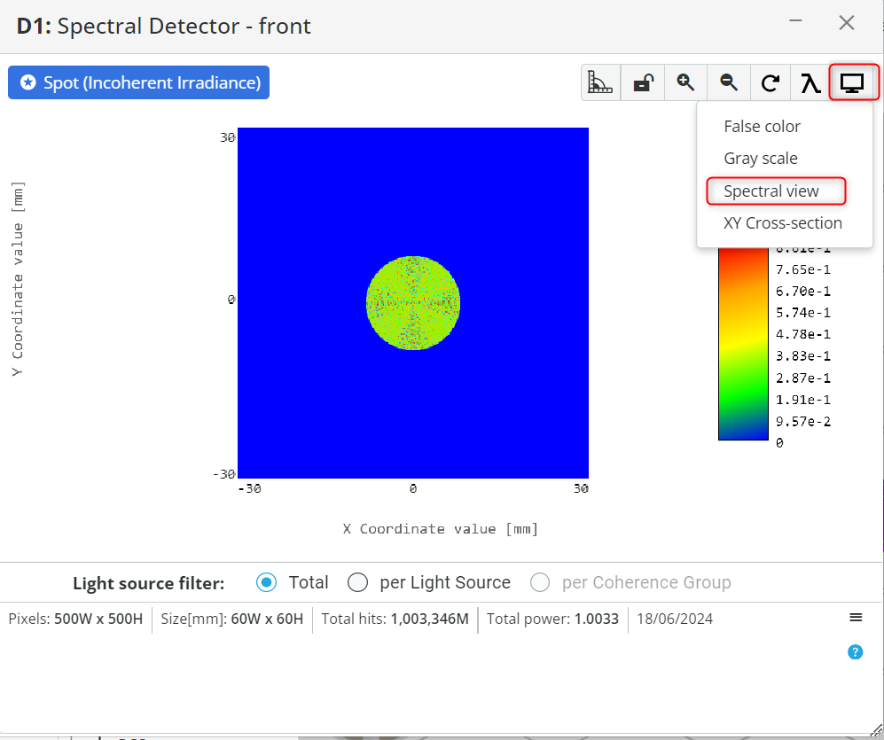
The detector setting is shown below while the detector is added by right-clicking on pane and selecting add detection.
  • Fill the Total spectral power table below:
Extra information
In the Czerny-Turner spectrometer, aberration correction is achieved through the strategic use of two concave mirrors: one for collimating incoming light and the other for precisely focusing dispersed light. This design effectively addresses spherical aberrations by ensuring that light rays remain parallel upon reaching the diffraction grating and are accurately focused onto the detector after dispersion. Additionally, careful alignment of the mirrors and selection of appropriate focal lengths help reduce astigmatism, which refers to variations in focal length for different meridians of the light beam. These optical adjustments contribute to maintaining high spectral resolution and accuracy in spectroscopic measurements. In more sophisticated configurations, aspheric mirrors replace spherical ones to improve optical performance. Aspheric mirrors excel in correcting higher-order aberrations, enhancing focus sharpness and resolution significantly.
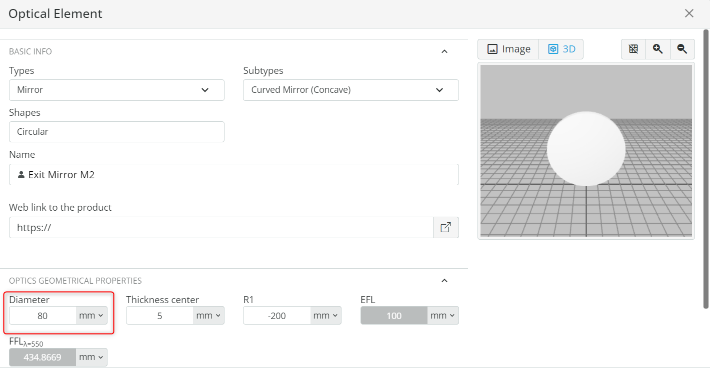
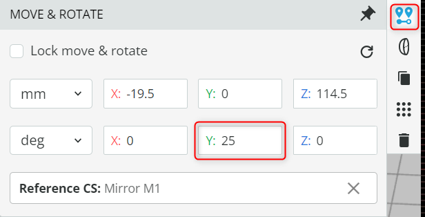
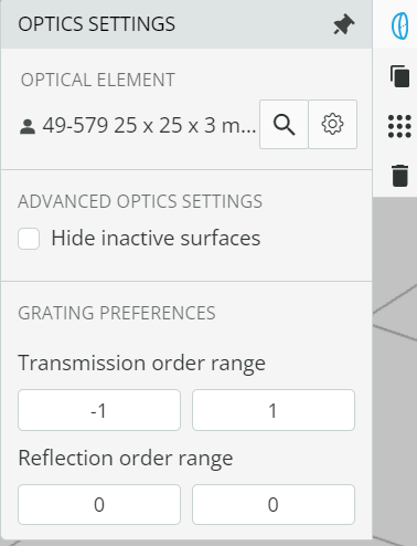
Exercise 3: Setting up grating and Exit mirror M2
  • Keep the file “Ex_2_CT_Spectrometer_Lens_ES_M1.opt” open.
  • Insert the grating 33009FL01-060R by opening the Product catalog. Reference the grating to the Mirror M1 and place the grating at the coordinates shown below.
  • Click on the Propagation simulation button. You will now observe a completely collimated light being reflected from the grating and a spectrum. You are supposed to observe the zero-order diffraction as a collimated light.
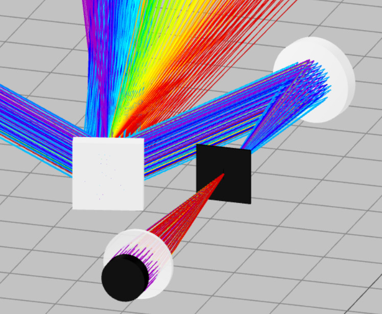
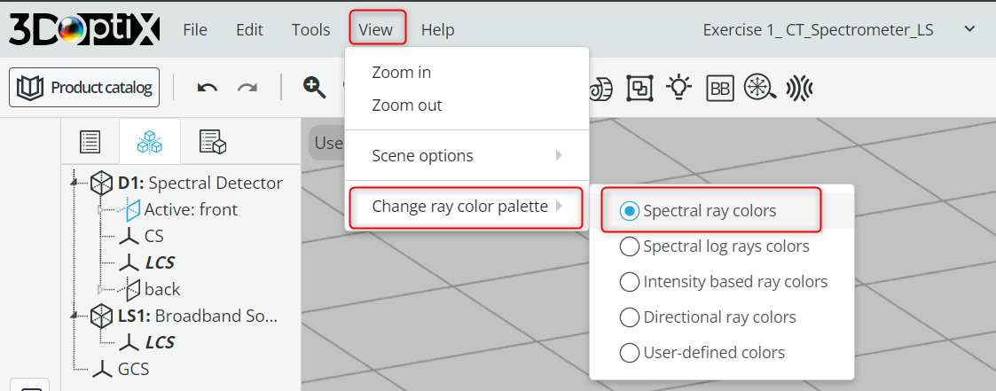
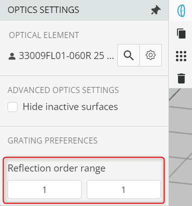
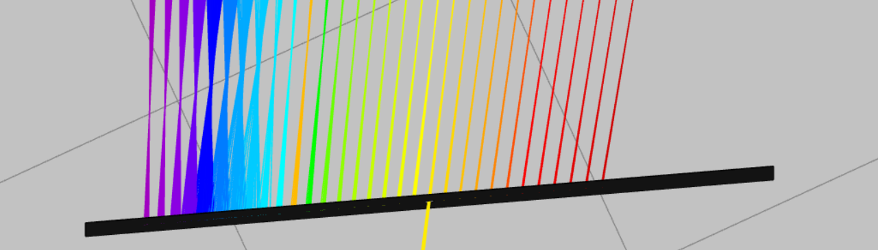
  • Hint: If you see multiple spectra compared to what is shown, then this means that you have enabled multiple reflection order range. You can change this using the method shown below.
  • Click on the grating and then go to the Optical settings available on the right side. Change the reflection order range from 1 to 1. This will choose only the first reflecting order of the grating.
  • Click the Propagation Simulation button. You should now see only the first-order dispersed spectrum.
  • Open the Optical Settings of the grating and under Optics physical properties, note down the Grooves/mm. Use this information for the tasks below.
  • Let us determine the basic performance parameters of the spectrometer using the equations mentioned below and note them down in the respective tables.
  1. Use the equation below to find out the divergence angle D_v and diffraction angle \beta for each wavelength defined. Choose the angle of incidence \alpha as 25 degrees and diffraction order m as 1.
    Note: This is a modified grating equation for the case when the incident light is not perpendicular to the grating normal, and the grating rotates around the plane that is coincident on its face.
mn\lambda = 2 \sin[\frac{(\beta + \alpha)}{2}]\cos[\frac{(\beta – \alpha)}{2}] where n=grooves/mm
D_v= \beta – \alpha
  • Now, let us capture all the dispersed spectra. Duplicate the Mirror M1 by first selecting it and then clicking the Duplicate option on the ribbon available on the right-hand side. This is shown below.
  • Rename the duplicated mirror to Exit Mirror M2. Then, open the Optical Settings of the Exit Mirror M2. Change the diameter of the mirror under Geometrical properties to 80mm and note down the effective focal length.
  • Place the exit mirror at the coordinates shown below. The mirror is referenced to the back side of the focusing lens. In this way, we have captured the entire spectrum from the first diffraction order. Click the Propagation simulation to confirm the result.
  1. Linear dispersion \frac{d\lambda}{dx} describes how the wavelengths are distributed along the spatial axis (usually the horizontal axis in spectroscopy). It is expressed in nm/mm. Use the equation below to determine the linear dispersion of the spectrometer for the diffraction angle calculated above.
\frac{d\lambda}{dx} = \frac{10^6\cos\beta}{mnf_b}
where f_b is the effective exit focal length of the mirror and dx is the unit interval in mm.
  1. Theoretical resolving power of a spectrometer is a measure of its ability to distinguish between two closely spaced wavelengths.
R = \frac{\lambda}{d\lambda} = mN = mnW_g = \frac{W_g(\sin\alpha + \sin\beta)}{\lambda}
Where d\lambda is the difference between two spectral lines of equal intensity (Spectral Resolution), N is the total number of groves and W_g=n*W is the illuminated width of grating, W is the width.
  • Calculate d\lambda using the equation above and enter the values in the table. Use the above recorded grooves density and illuminated width of grating as 22mm.
  1. The bandpass of a spectrometer is the range of wavelengths that can pass through the spectrometer’s entrance slit and be detected at a given wavelength setting. It is given by the following equation.
BP_{entrance} = \frac{10^6w_{entrance}×\cos\alpha}{mnf_a}
where w is the width of the entrance slit, f_a is the focal length of the collimating mirror
  • Open the Optical Settings on the user-defined object Entrance Slit. Note down the slit width. Now calculate the bandpass.
Extra information
“No single tool has contributed more to the progress of modern physics than the diffraction grating …”. [1]
“It is difficult to point to another single device that has brought more important experimental information to every field of science than the diffraction grating. The physicist, the astronomer, the chemist, the biologist, and the metallurgist, all use it as a routine tool of unsurpassed accuracy and precision, as a detector of atomic species to determine the characteristics of heavenly bodies and the presence of atmospheres in the planets, to study the structures of molecules and atoms, and to obtain a thousand and one items of information without which modern science would be greatly handicapped.” [2]
A reflective grating integrates a patterned structure onto a reflective surface, while a transmission grating incorporates a patterned structure onto a transparent surface. Master grating, also known as an original grating, is crafted directly from scratch using methods like mechanical ruling or holographic recording to form its surface-relief pattern. In contrast, a replica grating is produced by replicating the surface-relief pattern of another grating through casting or molding processes.
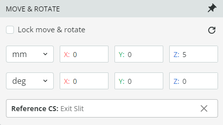
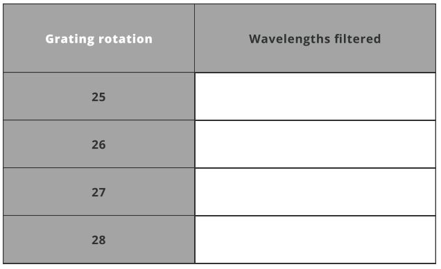
Exercise 4: Filtering spectrum, defining exit slit and detector
  • Keep the file open from Exercise 3.
  • At this stage, we will transform our spectrometer into a monochromator by introducing the Exit slit and defining the slit width. In addition, by changing the Exit slit width, we can change the bandpass.
  • Duplicate the entrance slit and name it “Exit slit”. Go to the optical properties of the user-defined object (Exit slit) and change the aperture settings. Change the half-width and half-height max to 25mm and set the Half-width and height min as shown. This is done to block the unwanted spectrum that may reach our detector.
  • Note: The instructions on how to duplicate an object and access the optical properties are shown in previous exercises. We will also change the Exit slit width later.
  • Change the coordinate of the exit slit as shown below. The exit slit is referenced to the Exit mirror. The exit slit is placed around 100m away from the mirror or at the focal length of the exit mirror.
  • Now place a detector right behind the exit slit. Reference the detector to the exit slit and place it at the coordinates shown. The detector has a half width and a height of 5mm.
  • There are two ways to filter the spectrum, either by changing the exit slit or by rotating the grating. Generally, a grating is rotated to filter the required spectrum. We will do both here. Change the width of the slit and record the spectrum by running the analysis in the analysis pattern.
  • Set the exit slit width min to 4mm and run the analysis under Analysis Portal.
  • Change the display of the detector from Spectral to false-color view and enlarge the detector by clicking on the detector window. Click on the false color detector view such that only the X-cross section view of the spectrum gets displayed, as shown below.
  • Calculate the Bandpass of the system using the data available through simulation. The bandpass of the system is calculated by the following equation:
BP=FWH × Dispersion
  • For simplicity, take only two spectral components and assume peak wavelength at our defined wavelength. Measure the wavelength difference d\lambda from the peak of the wavelengths. In our case, it is 10nm.
  • Use the cross-section view to measure the distance from the center of the 1st wavelength to the center of the second wavelength. This shows how far apart the two wavelengths are. Record this spread or increment dx from the cross-section image
  • Calculate dispersion by the following equation:
Dispersion = \frac{d\lambda}{dx}
  • Now calculate FWHM, and the BP
  • Calculate again the spectral resolution d\lambda using the detector pixel size \Delta{x} in mm by the equation shown below:
d\lambda = Dispersion \times \Delta{x}
  • Change the grating rotation angle as specified below and record the spectrum that is being filtered. For the exit slit, use a 4mm exit slit half-width. The rotation angle is changed by changing the parameter, as shown below.
  • Note that due to rotation, a few spectral components will not be blocked by the defined exit slit. In a real system, we must block all the rays that can cause stray light and hence degrade the system’s performance by introducing background noise.
Extra information
Invented in 1930 by Marcel Czerny and André Turner, the Czerny-Turner spectrometer was designed to enhance the performance and versatility of monochromators and spectrometers. This innovative configuration, featuring two mirrors, offers several advantages, such as reduced astigmatism and improved resolution, while its compact design minimizes aberrations and makes it suitable for a wide range of wavelengths. Due to its versatility and precision, the Czerny-Turner spectrometer has been widely adopted in both research and industrial applications, including chemistry, physics, astronomy, and material science. Over the years, the original design has been refined and adapted with advanced materials and detection technologies, further enhancing its performance and expanding its applications. The Czerny-Turner spectrometer remains a standard instrument in numerous laboratories today, continuing to serve as a fundamental tool for spectroscopic analysis. Its lasting relevance attests to the robustness and efficiency of the original design, cementing its legacy in the field of spectroscopy.
Experiment 2

Lens Grating Spectrometer

The lens grating spectrometer consists of two lenses, a collimating lens and a focusing lens, and a transmissive grating. Let us construct the lens grating spectrometer and analyze it.
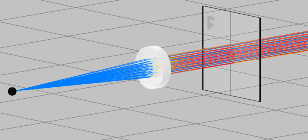
Exercise 5: Creating a divergence source and a collimating lens
  • Import the file “Ex_5_Lens_Grating_spectrometer_Src_Colli_Lens.opt” into the 3DOptix app.
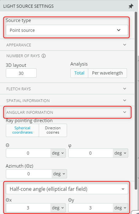
  • Go to the light source setting and under “Source type” see the definition of the source. In addition, see the angular information of the source. This indicates that we have a point source with a circular divergence of 6×6 degrees in both axes. Accessing the settings is shown in the above exercises.
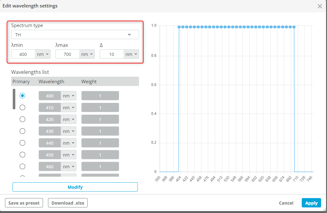
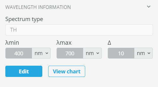
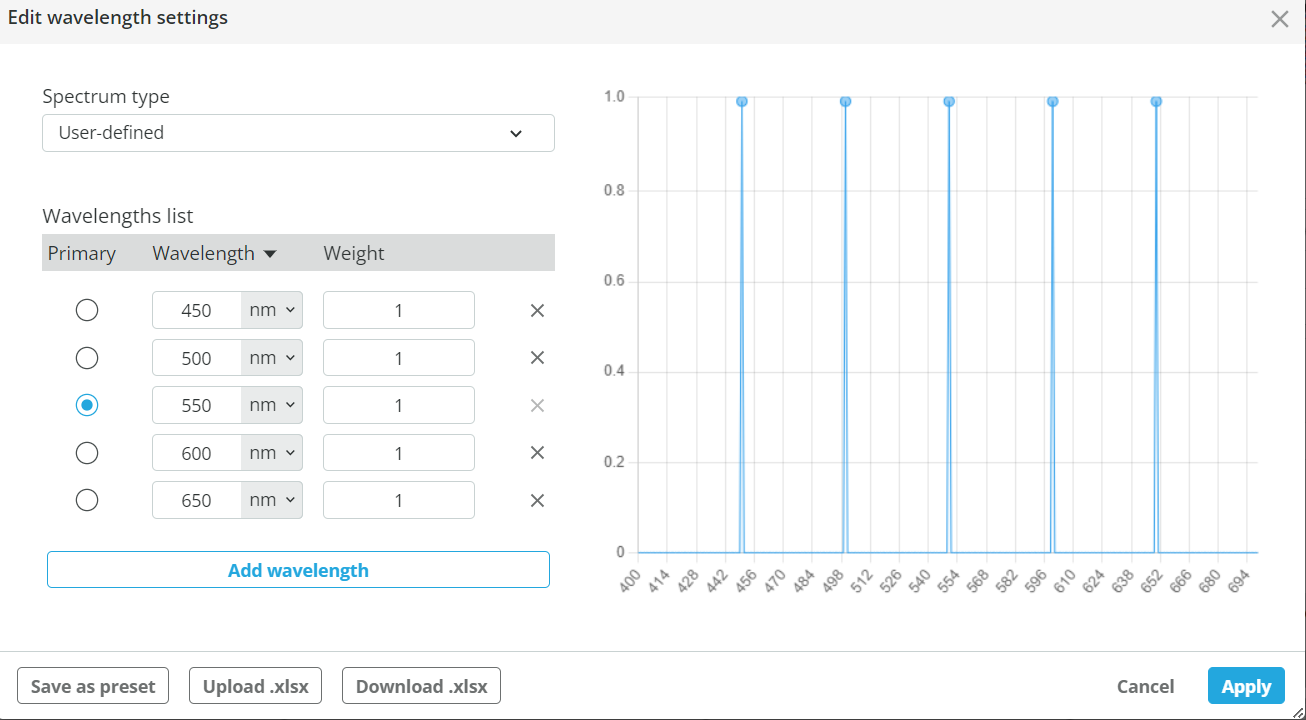
  • The source is then a polychromatic source (broadband) that consists of five wavelengths, separated by 50nm. Each wavelength has the same weight, and the central wavelength is 550. Don’t forget to hit the Apply button.
  • Collimate the light. Right-click on the Pane and add a user-defined object. Choose a lens with a subtype of Spherical Lens (Convex-Concave). Under Optics geometrical properties change the diameter to 10mm and R1 to 20mm. Note down the back focal length (BFL) and click save.
  • Now, using the lens maker equation, we can find out that to achieve collimation, the distance of the lens from the point source must be BFL. Set the coordinates of the collimating lens as defined below.
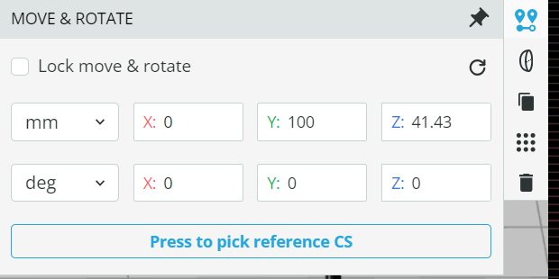
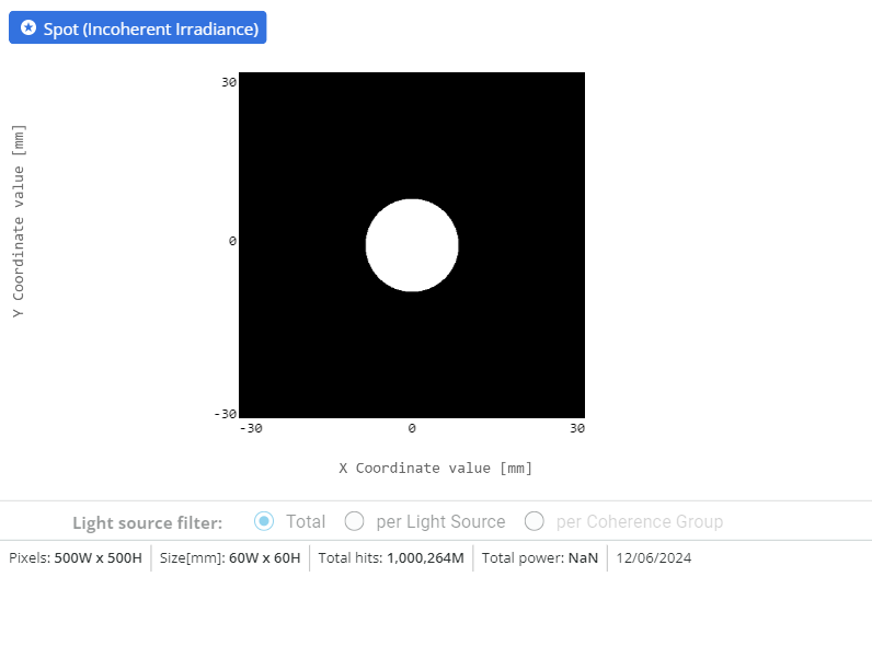
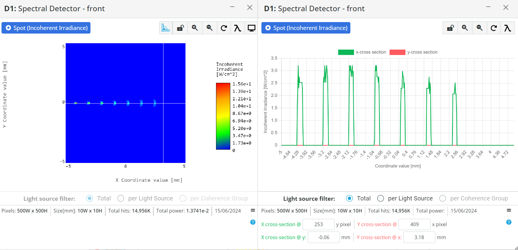
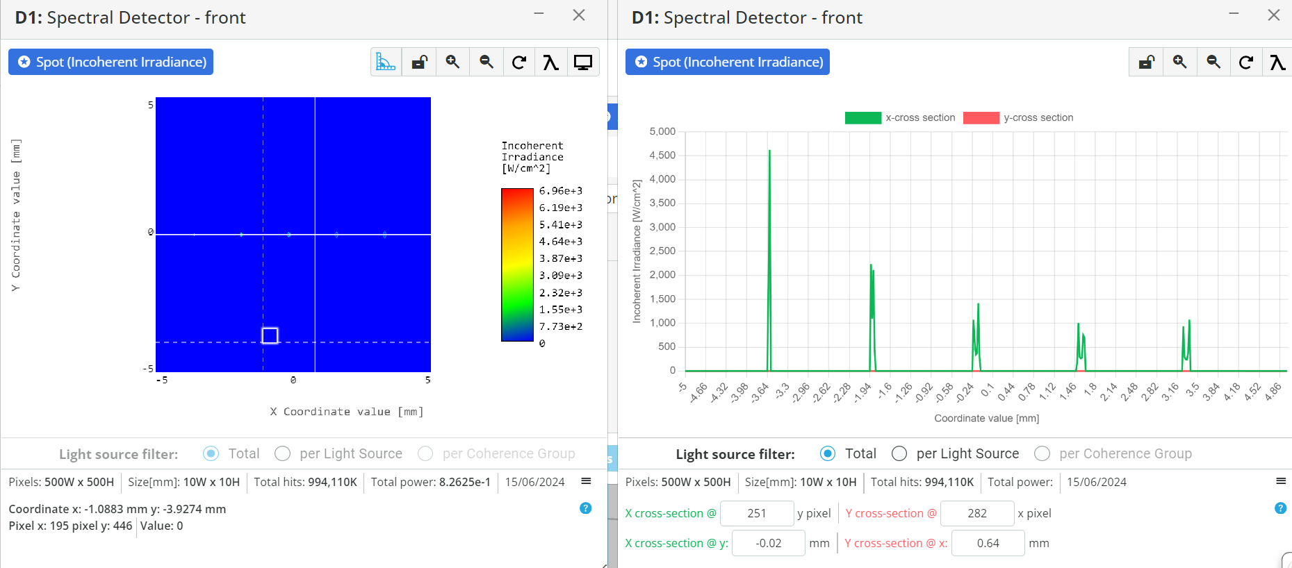
  • After setting the coordinate, add a detector in front of the lens and run the analysis in the Analysis portal to see the light output. Click the detector to enlarge it and click anywhere outside the output field to make a horizontal X-Cross-section. Write down the beam diameter = Do not put the detector too far away, as there will always be some divergence present in the system, and this will enlarge the output beam.
Extra information
Spherical aberrations in a transmissive grating spectrometer arise because spherical lenses cannot focus all incoming parallel rays to a single point. This optical flaw causes blurring of the spectral lines, diminishing the spectrometer’s resolution and accuracy. In such a spectrometer, light is diffracted by the grating and then focused by lenses. When these lenses are spherical, rays passing through the lens periphery focus differently than those near the center, creating a focal spread known as spherical aberration. To address this, aspheric lenses, which have a more complex shape than spherical ones, are often used to correct these deviations. These lenses enhance the focusing capability and overall performance of the spectrometer. Additionally, designing optical systems to minimize the incident angles on the grating can further reduce spherical aberrations. Precision in manufacturing and aligning optical components is crucial to managing these aberrations, ensuring the spectrometer delivers accurate spectral data.
Exercise 6: Setting up a transmission grating, a focusing lens, an exit slit and a detector
  • Keep the file “Ex_5_Lens_Grating_spectrometer_Src_Colli_Lens.opt” from previous exercise open.
  • Right-click on the pane and open the Product Catalog. Add a transmission grating (49-579) from Edmund optics. Under the optical settings of the element, note the grating density (grooves/mm). After that change the transmission order range of the transmission grating under optical settings.
  • Click on the Propagation simulation to see the spectrum. It must consist of 3 diffraction orders.
  • The diffraction angles are calculated using the equation mentioned below. Use m=1 for the first diffraction order and fill out the table. Take \alpha=0 for the collimated incident of light.
\beta = \sin^{-1}(\frac{\lambda}{d} – \sin\alpha)
where d is the distance between slit
d=\frac{1}{n}
where n is the grooves density
  • Now, let us focus only on the first order by turning off all the remaining orders. This is done by changing the transmissive order. Set the transmissive order to 1 and 1. Run the Propagation simulation and you will now see only 1st diffraction order.
  • Add a focusing lens to focus the first-order spectrum onto a detector. This is again done by adding another user-defined object by right-clicking on the pan and selecting the lens with the subtype as spherical lens (convex-concave). Set the optical properties as shown below. Reference the front side of the focusing lens with respect to the back side of the grating. The coordinates are shown below
  • Reference the detector with respect to the back side of the focusing lens and put the detector at the place where rays are focused. The detector size (X and Y half-width) can be changed to 5mm.
  • Run the analysis in the analysis portal and find out again the Bandpass of the system as shown in the exercise 5
BP=FWHM{\times}Dispersion=\underline{\quad\quad\quad\quad\quad}
  • Calculate again the spectral resolution d\lambda using the detector pixel size \Delta{x} in mm by the equation shown below:
d\lambda = Dispersion \times \Delta{x} = \underline{\quad\quad\quad\quad\quad}
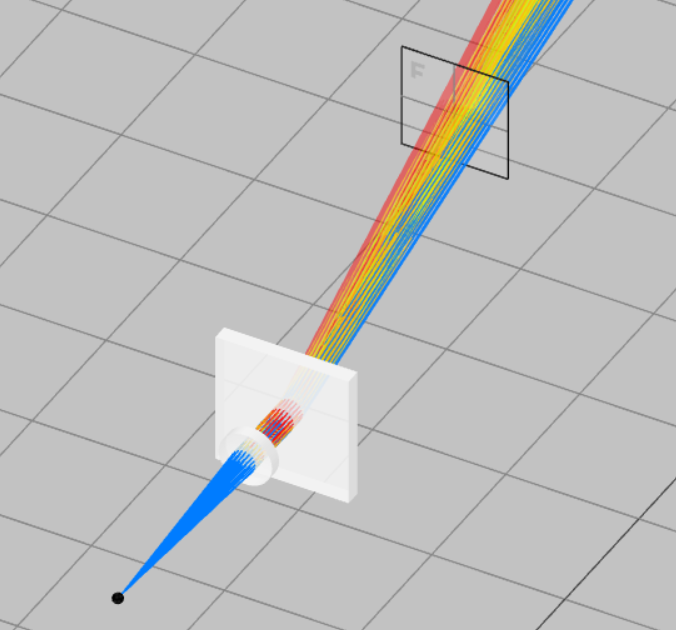
  • An exit slit can be placed after the focusing lens and before the detector to filter the desired wavelengths if required. 
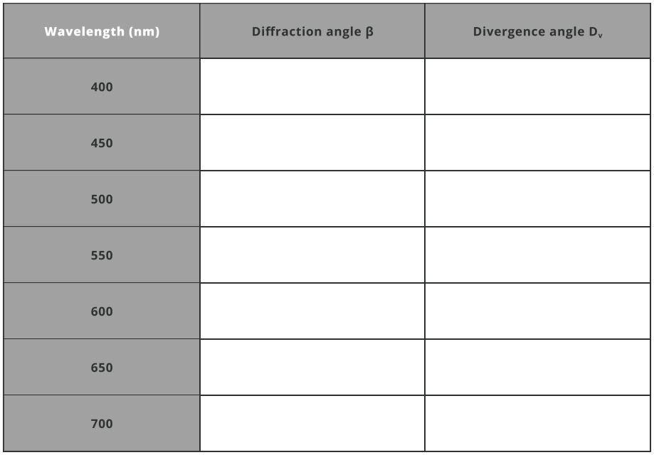
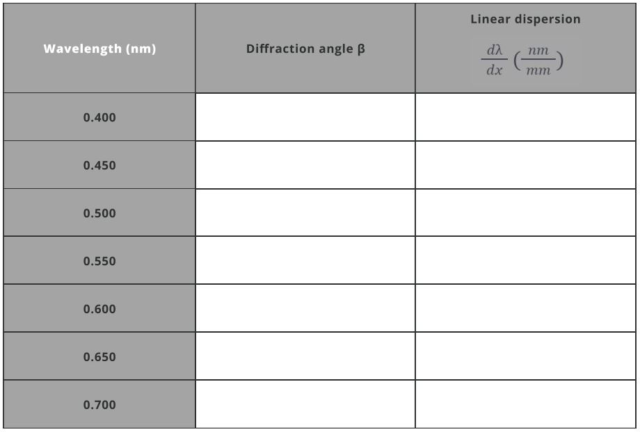
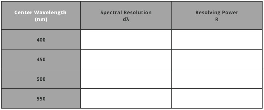
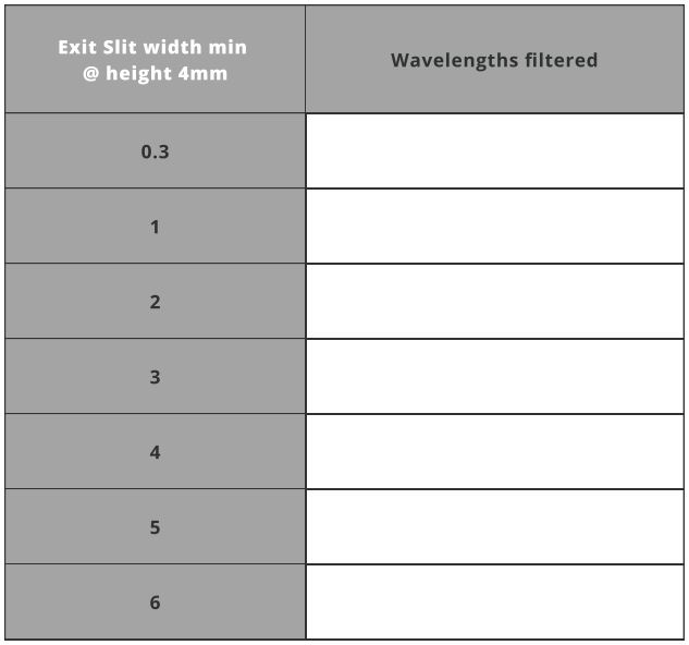
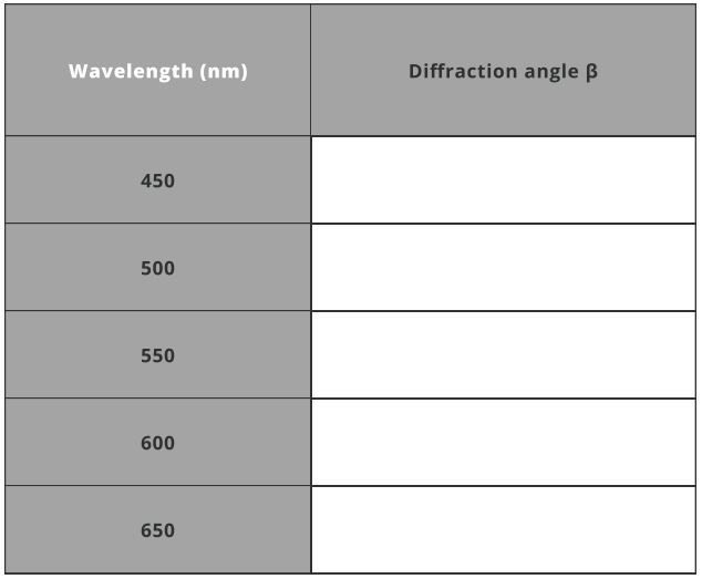
Filtered wavelength at defined parameters from the table below
Extra information
Transmissive and reflective gratings are crucial in spectroscopy, each suited for different applications due to their distinct characteristics. Transmissive gratings are commonly used in portable spectrometers and devices where light must pass through the grating. These include applications like environmental monitoring, quality control in manufacturing, and medical diagnostics. They are appreciated for their compact size, ease of integration, and cost-effectiveness, providing sufficient resolution for these purposes.
Reflective gratings, in contrast, are favored for high-precision and high-resolution applications. They can handle a wider range of wavelengths and are more efficient at higher diffraction orders. Reflective gratings are ideal for astronomical spectroscopy and essential for capturing faint light from distant stars and galaxies with high sensitivity. They are also used in advanced scientific research in material science and chemistry, where detailed spectral analysis is required. These gratings are best for situations where high spectral resolution and efficiency are more critical than size and weight.
In summary, while transmissive gratings are advantageous for compact, cost-effective applications, reflective gratings are the preferred choice for achieving high spectral resolution and efficiency in demanding scientific and astronomical contexts. The selection between the two types relies on specific application requirements, encompassing factors such as resolution needs, wavelength range, and budget considerations.
Analysis and Conclusion
Spectrometers play a crucial role in various fields of science, including astronomy, chemistry, physics, and biology. By analyzing the spectrum of a source, the nature of the object can be assessed. Therefore, this course covers not only the basics but also the detailed methods required to build and evaluate a spectrometer. Through hands-on construction and alignment of the Czerny-Turner and transmission (lens) grating spectrometers, students gained practical experience. The course enabled us to make spectrometers that measure the spectral lines of known sources, while also focusing on comparing the performance of both spectrometers, highlighting their applications and limitations in scientific research.
References
  1. G. R. Harrison, “The production of diffraction gratings. I. Development of the ruling art”, J. Opt. Soc. Am. 39, 413-426 (1949).
  2. J. Strong, “The Johns Hopkins University and diffraction gratings”, J. Opt. Soc. Am. 50, 1148-1152 (1960), quoting G. R. Harrison.
  3. MKS Diffraction Grating Handbook (8th edition).
  4. Handbook of Optical Systems, Volume 4 Survey of Optical Instruments by Herbert Gros.
  5. Laser Spectroscopy by Wolfgang Demtroeder.
Assessment
NA
Resources
The student requires an account in the 3DOptix system.
Synopsys
This lab involves the construction and analysis of two types of spectrometers: the Czerny-Turner spectrometer and the transmission (or lens) grating spectrometer. The Czerny-Turner spectrometer uses two concave mirrors and a diffraction grating to disperse light, while the transmission grating spectrometer employs lenses and a transmission grating. Students will align optical components to optimize bandwidth and assess the resolving power of both spectrometers. Additionally, the lab provides a detailed understanding of both theoretical and practical aspects of spectrometer development, offering hands-on experience in building these devices.
mascot-1-1

3DOptix works
only on desktop!

Please go to 3doptix.com on a
desktop device, using the
Chrome or Edge browser

Available on January 30th, 2023