Zoom Systems

VIRTUAL LAB

Zoom Systems

Course Overview
This pre-lab assignment aims to introduce students to the fundamental principles of fixed and variable zoom systems. Students will create different types of zoom systems, such as two-lenses and three-lenses zoom systems. A varifocal system, where the magnification changes dynamically by altering the focal length, will be analyzed and developed. During the analysis phase, students will gain a deep understanding of both design challenges and theoretical backgrounds. The course will address first design principles with paraxial lens analysis and then will replace the paraxial lenses with catalog lenses.
Course Duration
Approximately 3 hours (self-paced)
Learning Objectives
By the end of this pre-lab assignment, students should be able to:
  • Understand the basic principles of Zoom or varifocal systems
  • Layout the design criteria and development process of Zoom systems
  • Use analytical analysis to design zoom or varifocal systems
  • Explore the embodiment of the designed system and its limitation
  • Understand the design challenges and errors present in the system using simulations
Course Outline - Introduction to Zoom Systems:
A zoom or varifocal system is a specialized optical system featuring movable lens components or groups along the optical axis. This design allows continuous changes in focal length and magnification while keeping the image plane constant. The design and layout of such systems are complex, as they must perform well across the entire zoom range with minimal loss of image quality. While zoom systems are typically complex and contain many components, for educational purposes, we will focus on simpler systems with up to three lenses. In general, zoom systems can be classified into two types, as shown in the table below. Additionally, they can be characterized by different configurations, also shown in the table below.
Advancements in optical materials and computer-aided design have enhanced these systems, enabling higher image quality and greater versatility. Modern zoom systems are now integral to applications such as photography, microscopy, and telescopic observation, where precise control over magnification and image clarity is essential. Understanding the principles behind these systems is vital for developing effective and high-performing optical zoom solutions while also considering manufacturability and cost.

Basic Principles of Zoom Systems

Zoom System Types
Principle
Mechanically Compensated
Two or more components move relative to each other to change the focal length and magnification while keeping the image position constant.
Optically Compensated
A coupled part that may consist of multiple lens elements moves to change the focal length and magnification. Change of image location occurs in such systems.
Zoom System Configurations
Principle
Finite – Finite (F-F)
The Image and the object distances are located at finite position.
Infinite – Finite (I-F)
The object is located at an infinite distance and the image is at a finite location.
Infinite – Infinite (I-I)
Both the object and image are located at infinity. Complete afocal system.
A zoom system enables continuous variation of focal length, allowing the user to zoom in and out without moving the camera. The fundamental principles of a zoom lens system can be comprehended through lens formulas and geometric optics. Consider two thin lenses with focal lengths f_1 and f_2 are positioned at a distance t apart, the combined focal length of the system is given by:
f = \frac{f_1f_2}{f_1 + f_2 – t}
The lens formula from the thin lens equation where u is the object distance and v is the image distance is given by:
\frac{1}{f} = \frac{1}{u} + \frac{1}{v}
While the magnification of the lens is calculated by the equation:
M=-\frac{v}{u}
The total focal length for the two thin lenses is also given by the magnification m_2 of the second lens and the focal length of the first lens f_1
f=f_1m_2
One of the main considerations of a zoom system is the concept of the principle of the smallest change,  where we can avoid having long distances to move the components and achieve the required magnification. Therefore, we define zoom factor or zoom ratio, which for the case of Finite-Finite (F-F), is given by:
M=\frac{m_{max}}{m_{min}}
And for Infinite-Infinite afocal system it is given by:
M=\frac{\Gamma_{max}}{\Gamma_{min}}
\Gamma_{max} and \Gamma_{min} are the angular or telescopic magnification.
When two components are used and one is moved relative to the other to achieve the magnification, then the image location does not stay constant, therefore, two components’ movement is necessary to achieve a constant image distance.  In a more general case, three components are used, where two components are moving to achieve the variable magnification and the third lens stays stationary. In the case of three lenses design, four configurations are possible:
Possible configuration (3 Elements)
Fixed lens
plus-minus-plus
last lens
minus-plus-minus
last lens
minus-plus-minus
first lens
plus-minus-plus
first lens
In this lesson, we will focus on only plus-minus-plus, where the last lens is fixed.  In addition, the way the two lenses move can be defined by zoom curves. The zoom curves define the movement of lenses vs the magnification achieved. For several reasons, designing a zoom lens system is more complex than designing a fixed-focus system. It is difficult to achieve the desired zoom ratio while meeting requirements for overall length, mechanical constraints, and optical performance. There are several major considerations that should be taken into account in designing a zoom system:
  • Fixing imaging conditions.
  • Paraxial layout, length and power of the system.
  • Calculation of the lens movements and using minimum number of lenses.
  • Correcting aberrations over all the zoom range.
  • Cost, weight and size.
Experiment 1

Infinite – Infinite Two-Lenses Zoom System

In this experiment, we will be designing a fixed two-lenses beam expander. This beam expander can also be classified as a zoom system since an incoming beam gets magnified as it passes through the system. A Galilean two-lens beam expander uses a combination of a converging lens (with a positive focal length) and a diverging lens (with a negative focal length) aligned in sequence. The laser beam initially passes through the diverging lens and then the converging lens. The expansion factor is determined by the ratio of the focal lengths of the two lenses. This setup is compact, avoids creating an intermediate focus, and expands the beam while keeping it collimated.
Exercise 1: Setting up a source, a positive and a negative lens
  • Import the file “Ex_1_2Ls_I-I_ZS.opt” into the 3DOptix app. At this stage only a source is present.
  • Go to the light source settings and under “Source type” see the definition of the source. The source is a circular plane wave with a diameter of 2mm.
  • The source settings can be accessed by clicking on the source object. Then click on the “light source settings” option that appears on the ribbon available at the right-hand side of the source.
  • We keep the source monochromatic by defining only a single wavelength at 550nm. This setting is also accessible under the light source settings. A monochromatic source is defined to avoid the effects of Chromatic aberrations.
  • Right-click in the viewport and add a user-defined object. Choose a lens with a subtype of Spherical Lens (Concave-Concave). Rename it to “Negative Lens” and save it. This will add the lens.
  • Select the negative lens,reference it to the light source and put it at 10mm distance from the source. This is achieved by first accessing the ribbon on the right-hand side and clicking the Move/Rotate option. Then click the Press to pick reference CS. Afterwards select the Point source’s Local coordinate system (LCS) available on the left-hand side menu under Parts. The coordinates for the lens are shown below.
  • Right-click again in the viewport and add a user-defined object. Choose a lens with a subtype of Spherical Lens (Convex-Convex). Rename it to “Positive Lens”.
  • Reference the “Positive Lens” to the back side of the negative lens in the same manner as was done before. The coordinates for the positive lens are shown below.
  • Finally, add a detector by right-clicking in the viewport and reference it to the point source. The size of the detector can be changed by accessing the detector settings option available on the ribbon. Accessing detector and detector settings are shown below along with the detector coordinates.
  • At this point the system should have the following layout. We will adjust the distance and define the lens properties in the next exercise.
Extra information
A Galilean beam expander consists of a diverging (negative) lens followed by a converging (positive) lens. The incoming laser beam first goes through the diverging lens, which starts to diverge it, and then through the converging lens, which collimates the beam without an intermediate focus point. The magnification is determined by the ratio of the focal lengths of the two lenses. This setup is compact, simple, and generally more affordable. On the other hand, a Keplerian beam expander uses two converging lenses. The first lens focuses the incoming beam to an intermediate focal point, and the second lens then re-collimates and expands the beam. This design typically results in a longer optical path and a larger device but offers higher magnification and better beam quality. The Keplerian design is ideal for applications requiring high precision and minimal beam distortion despite being more complex and expensive. Both beam expanders are used to increase beam diameter for improved resolution or specific application needs, but they differ in their optical paths, design complexity, and practical benefits.
Exercise 2: Defining optical properties and embodiment information
  • Keep the file open from Exercise 1.
  • To define our beam expander or our fixed zoom system, we will use the Gullstrand’s equation that defines the effective power of the system.
{\phi} = {\phi_1} + {\phi_2} – {d} \times{\frac{\phi_1\phi_2}{n}}
  • Where \phi_1 and \phi_2 are the power of the first and second lens, while d is the distance between the two lenses and n is the refractive index. In this case n=1.
  • The effective focal length of the system is then given by:
\frac{1}{EFL} = \frac{1}{f_1} + \frac{1}{f_2} – \frac{d}{f_1 f_2}
  • Since for our case, when image is located at infinity EFFL = 0. This also defines a complete afocal system since our input beam is also parallel. The above equation further simplifies to:
0 = \frac{1}{f_1} + \frac{1}{f_2} – \frac{d}{f_1 f_2}


d = f_1 + f_2

  • In the case of thick lenses, we must take the lens thickness into account, which gives:
d = f_1 + f_2 – t_1 – t_2
  • The distance from the first lens surface of the negative lens to the last surface of the positive lens is defined as system track length TL and is given by:
TL = f_1 + f_2 + t_1 + t_2
  • The magnification power MP of the system is then given by:
MP = – {\frac{f_2}{f_1}}
  •  To define the radius of the lens, we will make use of the following equation:
\frac{1}{f_1}=(n_g – 1)\frac{2}{R_1}

\frac{1}{f_2}=(n_p – 1)\frac{2}{R_2}
  • Where n_g and n_p are the refractive indices of the negative and positive lens, while R_1 and R_2 are radii of the negative and positive lenses.
  • Fill the table below with the information provided. Assume t_1 = t_2 = 3mm. Find out the refractive indices under the optical properties of the lenses since the refractive index is dependent on the wavelength.
  • Access the optical settings of the negative lens and change its optics geometrical properties. This is done by right-clicking on the component and then clicking optical settings.
  • Change the “Z” coordinate of the negative lens to 15mm, as shown in Exercise 1.
  • Access the optical settings of the positive lens and change its optics geometrical properties.
  • Change the “Z” coordinate of the positive lens to -74mm, as shown in Exercise 1.
  • Click the Propagation Simulation button, which is available on the top right side.
  • Go to the Analysis portal and Run analysis. The detector settings are shown below.
  • Click on the detector window to enlarge it. Click on the detector outside the output field to draw the cross section of the beam. Measure the beam diameter with the measurement tool:
Beam Diameter  = ______________________________
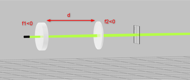
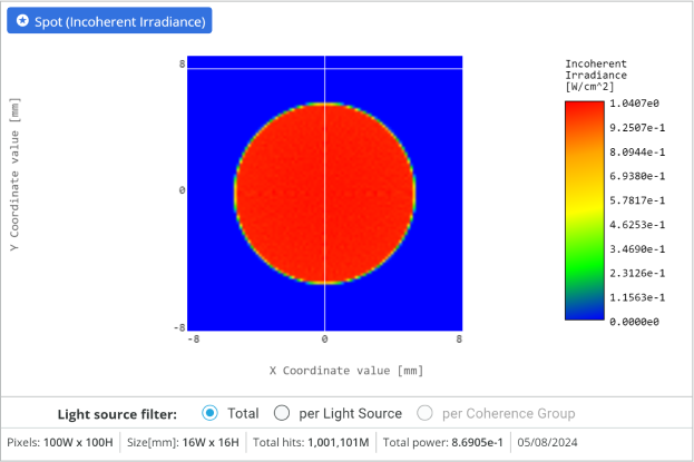
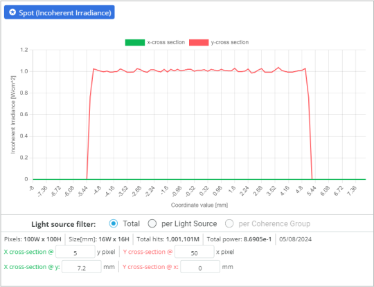
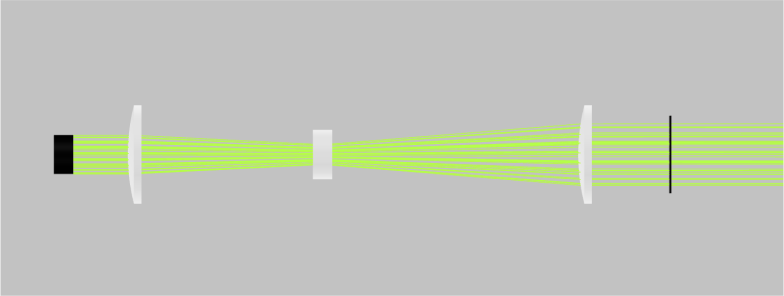
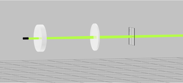
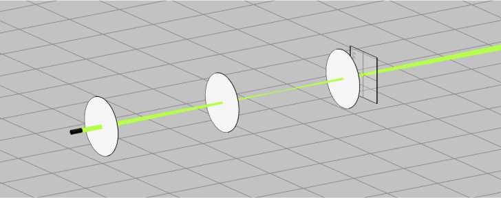
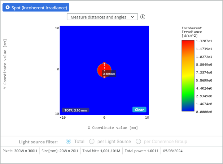
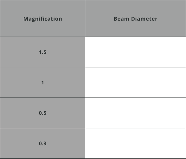
  • Although the beam is fairly collimated, the beam diameter is slightly larger. This is due to the fact that the beam has a small divergence and further optimization is needed. Try to reduce the beam diameter as close as possible to 10mm by changing the radii of two lenses or changing the distances between the lenses. 
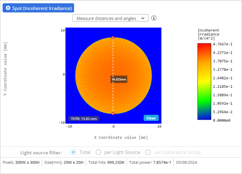
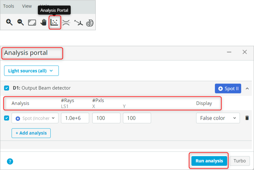
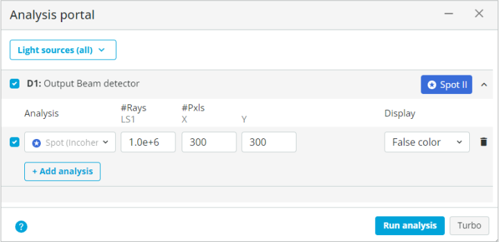
The number of detector pixels can also be changed to get a sharp beam profile output.
Extra information
A Galilean beam expander can experience several optical aberrations that degrade beam quality. Spherical aberration occurs when light rays passing through the lens edges focus differently than those near the center, resulting in a blurred image due to imperfect lens shapes. Coma aberration causes off-axis points to appear comet-shaped and asymmetrical, often due to lens surface imperfections or misalignment. Astigmatism stretches or blurs images in one direction, arising from differences in focusing horizontal and vertical rays due to imperfect lens shapes or misalignment. Field curvature makes flat objects appear curved, while chromatic aberration causes color fringes around images by focusing different wavelengths at different points. Distortion, either pincushion or barrel, alters the image shape, and any misalignment of optical elements can worsen these aberrations, further compromising the quality of the expanded beam. Careful design, precise manufacturing, and accurate alignment of optical components are essential to minimize these aberrations. To correct spherical aberration in optical systems like Galilean beam expanders, aspheric lenses with non-spherical surfaces are used to focus all incoming light rays to a common point. Another effective method is combining multiple lenses with varying curvatures to cancel out aberrations. Achromatic doublets, composed of two different types of glass, help correct spherical aberration and reduce chromatic aberration. Additionally, precision manufacturing and accurate alignment of optical components are essential to minimizing spherical aberration and enhancing overall image quality.
Experiment 2

Afocal (Infinite – Infinite) Three Lens Variables Zoom System

An afocal system consisting of three lenses provides a variable magnification by changing the distances between the lenses without the change of the focal lengths or the lenses. Maximum and minimum magnification can be defined. These correspond to a zoom factor. In the following, we will first build a paraxial system using analytical techniques and then replace it with the catalog lenses and do further optimization.
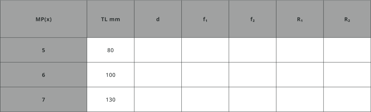
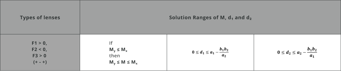
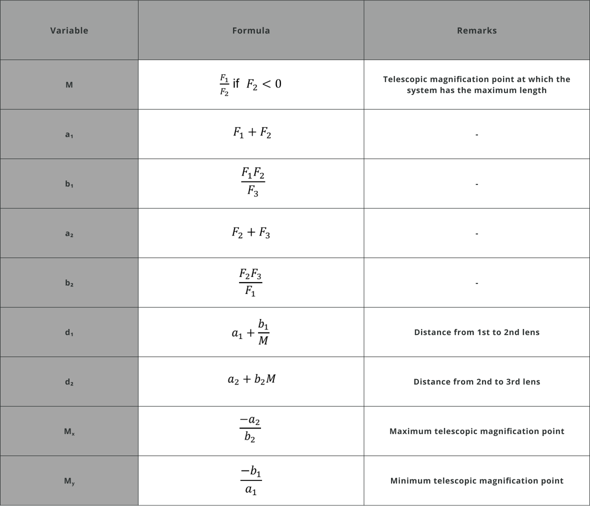
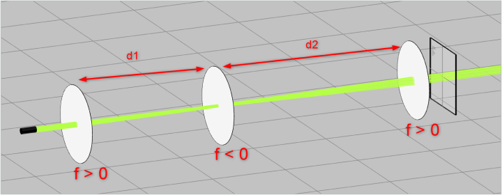
Exercise 3: Defining 3 lenses system - paraxial layout
  • Import the file “Ex_3_3Ls_I-I_Paraxial_ZS_Start.opt” into the 3DOptix app. The system contains an input beam, three paraxial lenses and a detector. Note the references of the components with respect to each other.
  • The source, lens placement, detector position and optical properties information can be found similar to the method as shown in exercises 1 and 2.
  • We will build a Plus/Minus/Plus beam expander where the last lens is fixed and calculate the required distances between the lenses to achieve the required magnification.
  1. The initial design and construction of zoom systems depend on paraxial analysis. In afocal zoom systems, it is necessary to determine the distances between optical components (lenses) to achieve the desired magnification height. Since the system is afocal, the output angle of the zoom system should be zero, resulting in an effective focal length of infinity. The distances between the lenses are calculated through the analytical formulae:
d_1 = f_1 + f_2 + \frac{f_1f_2}{Mf_3}
d_2 = f_2 + f_3 + \frac{f_2f_3M}{f_1}
  • where f_1, f_2 and f_3 are the focal lengths of three components, M is the telescopic magnification and d_1, d_2 are the distances from the first to second and second to last component respectively. Following relationship holds true for the telescopic magnification:
M > 1 \rightarrow Beam \space diameter \space reduction \space (demagnification)
M = 1 \rightarrow No \space magnification
M < 1 \rightarrow Beam\space diameter\space increases
  • Output beam diameter is then given by:
Output \space Beam \space Dia = \frac{Fill \space Input \space Beam \space height}{M}
  1. The solution space with a positive magnification of the system is shown on the table:
  1. Calculate the parameters shown in the table below and assume f_1 = 100mm, f_2 = – 20mm, f_3 = 100mm.
    NOTE: Negative lens distances must be discarded in practice, and the system’s magnification must be adjusted accordingly.
  1. In our case, we keep the last lens fixed and move the first two lenses. The system track length, which is the distance from the first to the last lens is given by:
TL = 2f_1 \times \frac{M_x-1}{M_x + 1}
  • Now change all the focal lengths of the paraxial lenses in the system as defined above. This is done by changing the optical properties of the lenses. After changing the properties of the lens, click Save to apply the setting.
  • Change the distances between the lenses for 0.64 magnification as calculated above. Exercise 1 and 2 shows how to change the distances (Z) between the lenses. The coordinates are shown below. See also the referencing of the lens components. Remember that the last lens is fixed at a distance of TL from the global coordinate at X = 0.
  • At this point the system should magnify the beam and the layout should look like this
  • Go to the Analysis Portal and run the analysis. The detector settings are shown below.
  • Click to enlarge the detector and measure the beam diameter.
  • Measure again the beam diameter for the magnifications defined below.
  • Plot the distances d_1 and d_2 vs. the magnification value. Add the plot below inside the box available. The plot shows the zoom curves. Change in magnification with the change in distances between the lenses.
  • The distances can also be plotted from a reference origin where the first lens is at the origin and the last lens is at the location of the TL. For such a case, we need to make a minor change and the distances then become:
t_{2_{mod}} = TL \medspace – \medspace d_2
t_{1_{mod}} = t_{2_{mod}} \medspace – \medspace d_1
  • As an example for the above system, the zoom curves are also shown below
Extra information
In designing a zoom system, zoom curves are essential for smooth and precise transitions between focal lengths. Key design considerations involve choosing the right lens elements and configurations to achieve the desired zoom range and image quality. Ensuring the smoothness of zoom curves is critical for maintaining consistent focus and image clarity, requiring meticulous engineering and calibration. Mechanical aspects focus on the durability and reliability of moving parts, ensuring lens groups move seamlessly without causing wear or misalignment over time. Cost and budget are also important, as high-quality zoom curves often demand advanced materials and manufacturing techniques, which can drive up production costs. Striking a balance between these factors is crucial to developing a zoom system that offers excellent performance and longevity while staying within budget. This balance ensures that the zoom system meets high optical and mechanical standards, making it suitable for both professional and consumer use.
Exercise 4: Replacing paraxial lens with catalog lenses
  • Keep the file open from the previous exercise number 3.
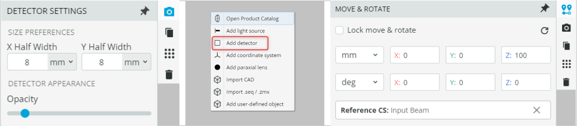
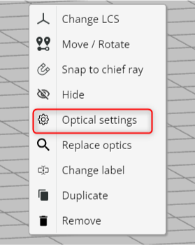
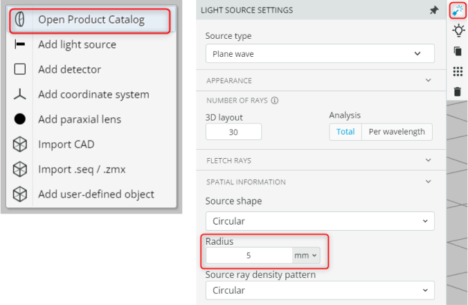
  • Change the spatial information of the source to Radius = 5mm. Replace the paraxial lenses with the catalog lenses. This is done by deleting the paraxial lens and adding the catalog lens from the product catalog.The product catalog is accessed by right-clicking on the Pane and selecting Open Product Catalog and then searching for the required part.
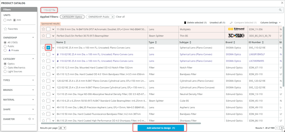
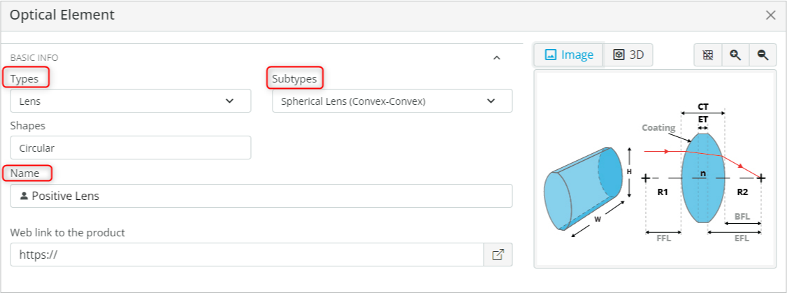
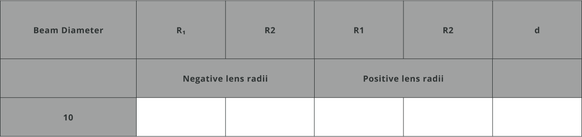
  • Replace the paraxial lenses with the following catalog lenses:
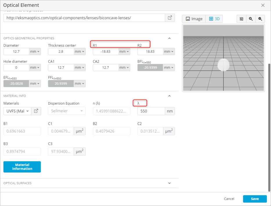
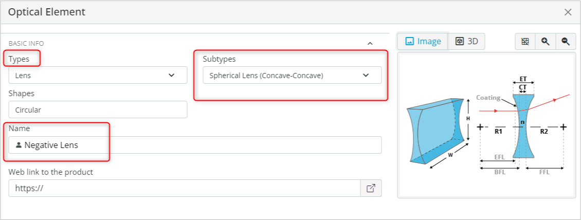
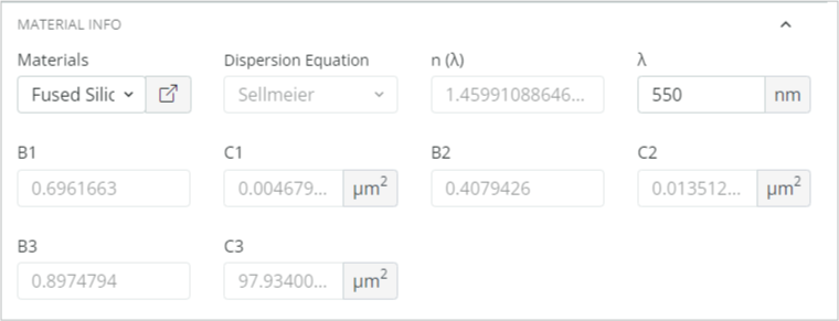
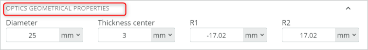
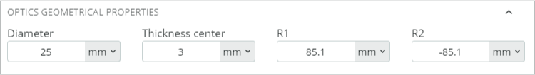
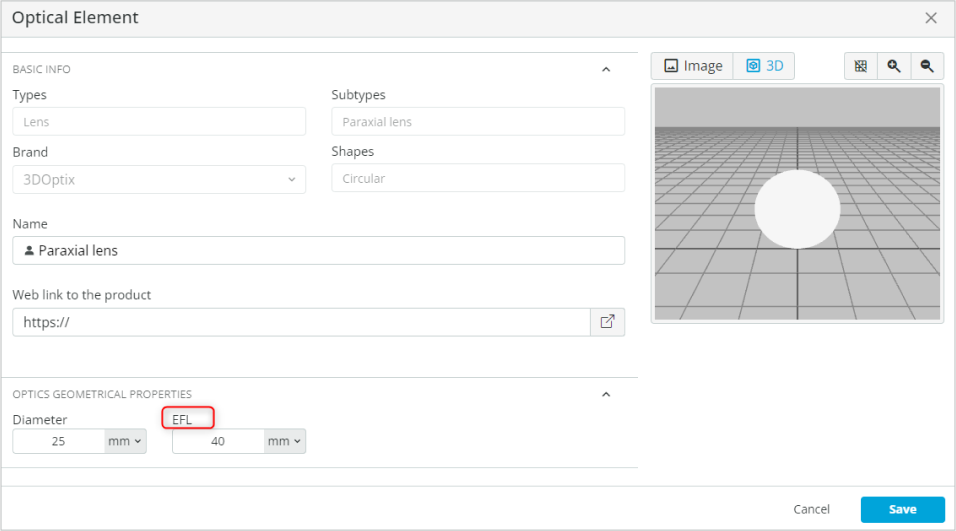
    • f_1=f_3=100mm= 110-0219E
    • f_2=-20mm=114-1108E
    • Access the Optical settings of the f_2 lens, rename it to “Neg_114-1108E 12.7 mm Dia. x -20 mm FL; Uncoated; Double-Concave Lens”, change the radii and wavelength as shown below.
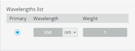
    • For f_1, f_2 and f_3 change the wavelength info to 550nm.
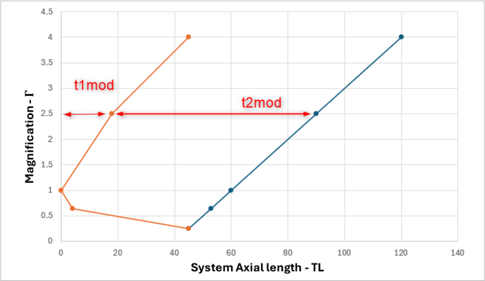
    • For the 0.64x telescopic magnification, specify the distance between the lenses as calculated above.
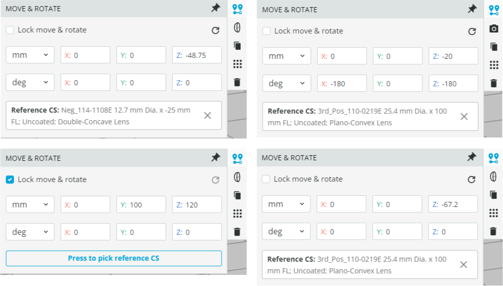
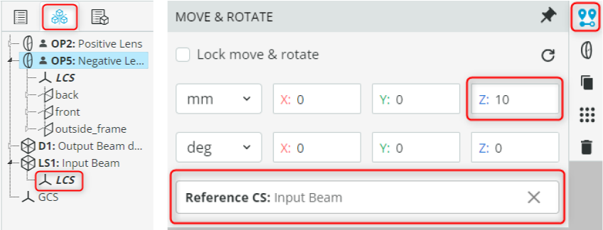
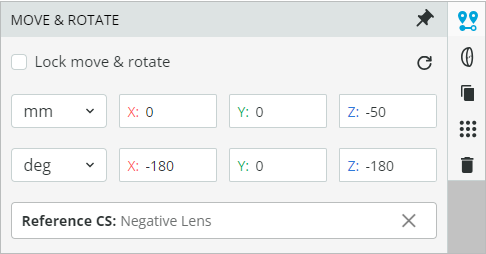
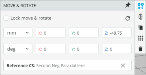
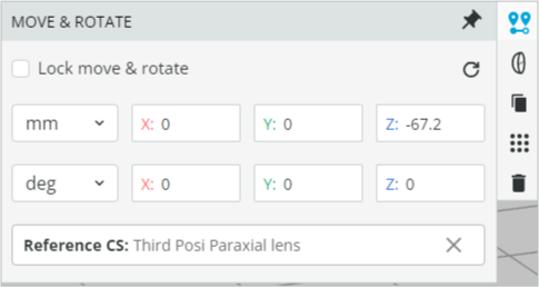
    • The first lens (front surface) is referenced to the second lens (front surface), and the second lens (front surface) to the last lens (front surface). While the third lens (front surface) is fixed at 120mm. The references and the coordinates are shown below.
    The detector is referenced to the front surface of the first lens.
  • Click on Propagation Simulation. At this point your system should look like this:
  • Go to the Analysis portal and run the analysis. Click on the detector to enlarge the detector window and measure the beam diameter: ____________________
  • The beam is still fairly collimated even after the introduction of thick lenses. The beam can be further collimated by a combination of changing the distances, modifying the radii of the lenses and flipping the lenses.
  • It should be noted that achieving the collimated beam is not enough. Certain applications require that the output beam is free of aberrations and is diffraction limited. Wavefront error less than λ/4 or more.
Extra information
A spot diagram can be used to evaluate a system’s performance. The Spot diagram is a two-dimensional distribution of ray pierce in an image plane obtained by superimposing pupil ray distribution(s) grid over the entrance pupil and launching rays from the off-axis points of an object to pierce the grid points in the pupil. These rays emerge into image space and converge toward the image plane. Aberrations in an optical system depend on the distribution of the ray’s pierce. The compact spot on the spot diagram represents less system aberrations. A quick check to evaluate the system performance is to compare the system’s spot size with a spot size from an ideal system known as Airy disk. If the spot size of a system is under the diameter of the Airy disk, then the optical performance of the system can be considered diffraction-limited. The expression for the Airy disk is given as:
D = 2.44 \times \lambda \times (f/{\#})
Where D is the physical diameter of the Airy disk, \lambda is the wavelength and (f/\#) is the F-number defined as the ratio of the system’s focal length over the diameter of the entrance pupil.
Analysis and Conclusion
A zoom system provides the ability to adjust focal length continuously, enabling users to zoom in and out without repositioning the camera. This flexibility is essential for capturing different perspectives and details in applications such as photography, microscopy, and telescopic observation. It enhances versatility and convenience, making precise control over magnification critical for many optical tasks. Therefore, the course covered not only the basic theoretical considerations but also the detailed methodology required to build and evaluate such systems. Students gained practical experience by constructing the zoom systems and achieving different magnifications by changing the optical parameters and distances. The performance of the systems was also addressed, which highlighted a different perspective on the evaluation of the system.
References:
  1. Handbook of Optical Systems, Volume 4 Survey of Optical Instruments by Herbert Gross
  2. Yeh, M.-S., Shiue, S. G. and Lu, M.-H., “First-order analysis of a three-lens afocal zoom system”, Optical Engineering 36(4) (1996)
  3. Yeh, M.-S., Shiue, S. G. and Lu, M.-H., ” Two-optical-component method for designing zoom system”, Optical Engineering 36(4) (1995)
Assessment
NA
Resources
The student requires an account in the 3DOptix system.
Synopsys
This lab involves the construction and analysis of two types of zoom systems: the two-lenses afocal Galilean beam expander with a fixed magnification and the three-lens afocal variable zoom system. With a three-lenses system, a change of magnification is achieved by varying the distances between the two lenses, unlike with a two-lenses system, where only a fixed magnification is possible. The students will build zoom systems using analytical techniques and then further optimize the output when paraxial lenses are replaced with catalog lenses. Additionally, the lab provides a detailed understanding of both theoretical and practical aspects of zoom systems, including the design challenges. This offers hands-on experience in building such sophisticated systems.
mascot-1-1

3DOptix works
only on desktop!

Please go to 3doptix.com on a
desktop device, using the
Chrome or Edge browser

Available on January 30th, 2023